The aim of this paper is to review the most important methodological strengths and limitations of observational studies of humans, as opposed to experimental studies. The names “observational” and “experimental” go a long way in describing the differences. In an experimental study—that is, a randomised controlled trial (RCT)—the investigator experiments with the effect of the exposure by assigning exposure to a random sample of the study subjects. In an observational study, on the other hand, the investigator can only observe the effect of the exposure on the study subjects; he or she plays no role in assigning exposure to the study subjects. This makes observational studies much more vulnerable to methodological problems, so it is only reasonable that RCTs are considered the best way of proving causality.¹

One might ask why all studies are not experimental. First, not all research questions are suitable for an experimental design. Studies of diagnostics tests and treatment are highly suited, but studies of drug effects in pregnant women, or of the prognostic impact of diseases, are among the research questions that cannot be studied in an experimental design. Second, RCTs are often very expensive, in terms of both time and money, and an RCT may be conducted only after observational studies have failed to provide a clear answer to the research question. Observational studies give an idea about the incidence, prevalence, and prognosis of the disease that is studied, and this information is necessary for proper planning of the RCT. Often, the RCT will confirm what has been found in the preceding observational studies,^2,3 but occasionally the findings differ, or are even in the opposite direction, as in recent studies of the effect of hormone replacement therapy on cardiovascular risk.^4–6

Consequently, most research questions will be addressed in one or more observational studies, so it is highly relevant for all physicians to be able to critically interpret findings from such studies.

ASSOCIATIONS

In clinical epidemiology, the two basic components of any study are exposure and outcome. The exposure can be a risk factor, a prognostic factor, a diagnostic test, or a treatment, and the outcome is usually death or disease. In an observational study, the frequency of an outcome—or an exposure, depending on the study design—is measured, estimated, or visualised. Risks, rates, prevalences, and odds are common measures of the frequency of an outcome, and comparing them between groups will yield relative frequency measures—that is, relative risks, rate ratios, prevalence ratios, and odds ratios. These describe the association between exposure and outcome and provide the basis for the study’s conclusions.

Surrogate measures

If the outcome of interest is disease, the actual study outcome is sometimes a surrogate measure for the disease. Surrogate measures are often used when the disease is so rare or so far in the future that it would take an unreasonably long follow up period to obtain a sufficient number of outcomes.

• Example—In the Los Angeles atherosclerosis study, Nordstrom and colleagues examined the three year progression of intima–media thickness of the carotids in a group of 40 to 60 year olds. Exposure groups were defined by the degree of physical activity. The authors found that intima–media thickness, a surrogate measure for cardiovascular morbidity, was inversely related to the degree of physical activity.⁷

Hypertension and hyperlipidaemia are among the most frequently used surrogate measures for cardiovascular disease, but even though the association between the surrogate measure and the true outcome may be biologically plausible, using the surrogate measure may produce misleading results if the association with the true outcome is not based on empirical evidence.^8,9

OBSERVATIONAL STUDY DESIGNS

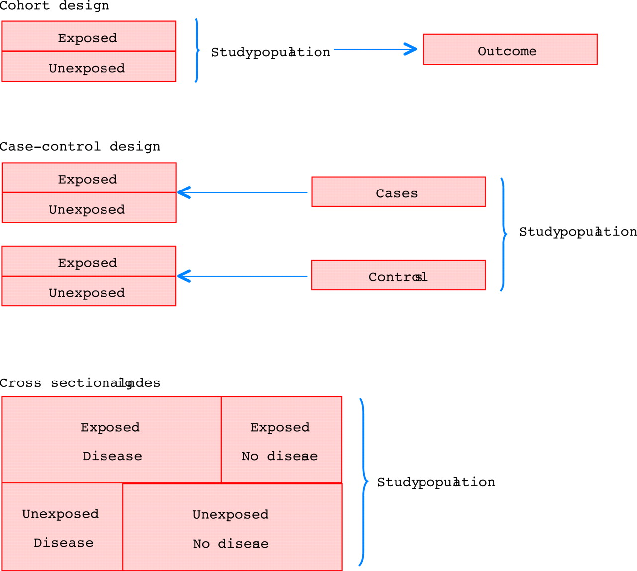
Three main study designs are used in observational studies: cohort (follow up), case–control, and cross sectional designs (fig 1).¹⁰

Cohort design

In a cohort study, patients with different levels of exposure are followed forward in time to determine the incidence of the outcome in question in each exposure group. With this design, the investigator can study several outcomes within the same study, and the most common frequency measures are relative risks, incidence rate ratios, and excess risks. If the outcome of interest is rare, a very large study population must be followed to observe a number of outcomes that is sufficient to demonstrate a precise association between the exposure and the outcome—that is, that will rule out chance as an explanation for the observed findings.¹⁰

Case–control design

In a case–control design, the first step is to identify those with the outcome of interest—the cases. That makes it a good design for studying rare outcomes, which would require a huge sample size in a cohort design, and this means that case–control studies are generally cheaper, too.¹⁰ Having identified the cases, the investigator selects the controls from the source population. There are a number of methods of doing this, but, regardless of the method, the level of exposure is compared between cases and controls. The relative frequency measure is the odds ratio, which is an estimate of the relative risk. The estimate is better if the disease is rare,⁸ but still the odds ratio will be biased away from the null—that is, it will be further from 1.0 than the relative risk, in studies of a dichotomous outcome. Using a nested case–control design and the incidence density sampling technique, however, allows the investigator to assume that the odds ratio is an unbiased estimate of the incidence rate ratio. A nested case–control study is actually a case–control study set within a cohort study, and the point of incidence density sampling is that controls are selected so that they have the same time at risk as cases.

Cross sectional design

Studies with a cross sectional design are also called prevalence studies.¹¹ With this design, exposure and outcome are measured simultaneously. Prevalence rates can be compared between groups, but the terms “exposure” and “outcome” are treacherous because the sequencing of the two is impossible to assess.¹⁰ Therefore, a cross sectional study is generally used to provide the basis for a subsequent cohort study, case–control study, or RCT.

REASONS FOR ASSOCIATIONS

There are four principal reasons for associations in an epidemiologic study: bias, confounding, chance, and cause. An essential aim of the design and analysis phases is to prevent, reduce, and assess bias, confounding, and chance, so that a causal unbiased association between exposure and outcome is estimated.¹⁰

BIAS

Bias means that a measure of association between exposure and outcome is systematically wrong. Evaluation of bias is a two step process: first, the investigator must determine whether bias is present; and then, second, consider its magnitude and direction. Usually, epidemiologists talk about bias away from the null and bias towards the null, meaning that the reported measure of association is systematically overestimated or underestimated, respectively. The two main types of bias are selection bias and information bias.

Selection bias

Selection bias relates to the design phase of an observational study, and it is more common in case–control studies than in cohort studies. In a case–control study, the investigator selects cases and controls that represent a source population, and the only intended difference between the two groups is the outcome. Selection bias occurs if the selection process introduces another, unintended systematic difference between the groups, and this systematic difference is associated with the exposure. In other words, the apparent association between exposure and outcome in a biased case–control study is in fact a combination of the association between exposure and outcome and the association between being selected as a case or control and the exposure.¹² Selection bias can be either towards the null or away from the null.

• Example—Using a case–control design, von Eyben examined smoking as a risk factor for myocardial infarction. Cases were patients with a myocardial infarction between 1983 and 1997, and controls were selected among patients admitted with inguinal hernia and acute appendicitis in 1990–1996. In 1997, both groups were asked in a questionnaire about their smoking habits, among other things, and the authors reported that smoking increased the risk of myocardial infarction. However, 27 of 77 patients with acute myocardial infarction had died at the time of the questionnaire, and, as the authors pointed out, that might have introduced selection bias; the possibility of being available at the time of the questionnaire is an unintended systematic difference between cases and controls, and it is also related to smoking. In other words, as above, the apparent association between smoking and myocardial infarction is a combination of the association between smoking and myocardial infarction and the association between smoking and being available at the time of the questionnaire. The resulting bias is presumably towards the null because it is likely that those who smoked less had a higher possibility of being available at the time of the questionnaire than those who smoked more.¹³

In a cohort study, selection bias occurs if the investigator’s selection of exposed and reference groups introduces a systematic difference, other than the exposure, between the groups, and this systematic difference is associated with the outcome.

Information bias

In a cohort design, an error in measuring exposure or outcome may cause information bias. Non-differential misclassification is seen when the errors in classification of exposure or outcome are random. An example of non-differential misclassification is the misclassification caused by coding errors due to accidental mistyping. In contrast, differential misclassification in a cohort study is when the degree or direction of misclassification depends on exposure status, or other variables.¹¹ In RCTs, this is avoided by standardised outcome assessment and blinding to exposure status. Non-differential misclassification will usually lead to bias towards the null, whereas differential misclassification can lead to bias in either direction.¹²

In a case–control study, cases and controls may have different degrees or directions of misclassification of exposure—that is, differential misclassification. This is of particular concern when exposure status is self reported, in which case a bias is called recall bias.

• Example—Tzourio and colleagues used a case–control study to examine whether migraine is a risk factor for ischaemic stroke in young women. Cases were women under 45 years of age with ischaemic stroke, and controls were randomly selected women with orthopaedic or rheumatological illnesses. Cases and controls were interviewed about headache, and other factors, and the authors found an odds ratio of 6.2 for ischaemic stroke among women with migraine with aura. Perhaps this was due to recall bias; cases may have been more aware of signs and symptoms that might explain their stroke.¹⁴

CONFOUNDING

Confounding is about the characteristics of the study subjects; patients with certain characteristics tend to have certain exposures. The aim of an observational study is to examine the effect of the exposure, but sometimes the apparent effect of the exposure is actually the effect of another characteristic which is associated with the exposure and with the outcome. This other characteristic is a confounder, provided that it is not an intermediate step between the exposure and the outcome.⁸ Therefore, a high cholesterol value should not be treated as a confounder in a study of the risk of coronary heart disease (outcome) in patients with severe obesity (exposed group) and patients with normal weight (reference group); although a high cholesterol value is associated with both obesity and coronary heart disease, it is an intermediate step because it may be caused by obesity.

There are two principal ways to reduce confounding in observational studies: (1) prevention in the design phase by restriction or matching; and (2) adjustment in the statistical analyses by either stratification or multivariable techniques. These methods require that the confounding variables are known and measured. In an RCT, on the other hand, the randomisation process allows the investigator to assume that not only known, but also unknown, potential confounders are distributed evenly among the exposed and the unexposed. Therefore, they are not associated with the exposure, hence they cannot be confounders.

Restriction

Confounding can be reduced by restricting the study population to those with a specific value of the confounding variable.¹² This method, also known as specification,¹⁰ makes examinations of the association between the confounder and the outcome invalid, and the findings cannot be generalised to those who were left out by the restriction.

• Example—Ayanian and colleagues examined the effect of specialty of ambulatory care physicians on mortality after myocardial infarction in elderly patients. They found that patients who saw a cardiologist had lower mortality than patients who saw an internist or a family practitioner. They excluded patients who died within three months, patients with metastatic cancer or a do-not-resuscitate order, patients who enrolled in a health maintenance organisation, patients residing in nursing homes, patients who lacked Medicare part B coverage, and patients with no ambulatory visits. These restrictions could serve to reduce confounding from the degree of morbidity, as the moribund and the, presumably, perfectly well patients, with no need for ambulatory visits, were excluded.¹⁵

Matching

Matching constrains subjects in different exposure groups to have the same value of potential confounders, often age and sex.¹⁰ However, with increasing numbers of matching variables, the identification of matched subjects becomes progressively demanding, and matching does not reduce confounding by factors other than the matching variables. Matching is most commonly used in case–control studies, but it can be used in cohort studies as well.

• Example—In a study of predictors of peripheral arterial disease, Ridker and colleagues nested a case–control design in the Physicians’ Health Study cohort, consisting exclusively of men. They identified 140 cohort members who developed peripheral arterial disease (cases). Controls were selected with the incidence density sampling technique and matched on age and smoking status to reduce confounding by these variables. The matching variables, the 11 candidate predictors, and remaining confounders (hypertension, body mass index, family history of premature atherosclerosis, diabetes, and exercise frequency) were then included in a multivariate model. The authors concluded that the total cholesterol/high density lipoprotein cholesterol (TC/HDL-C) ratio and C reactive protein (CRP) were the strongest lipid and non-lipid predictors of peripheral arterial disease.¹⁶

Stratified analysis

Stratification means that the study population is divided into a number of strata (subsets), so that subjects within a stratum share a characteristic, and each stratum is analysed separately. If the study population is to be divided into more than a few strata, it has to be large to begin with to yield conclusive results. Stratified analyses are the best way to evaluate effect modification (see below), but they are also a way of examining, or adjusting for, confounding. Confounding can be adjusted for if the strata are recombined with the Mantel-Haenszel method or a similar method.⁸

• Example—Ridker and colleagues studied whether CRP would improve prediction of risk of myocardial infarction. They used data from the Physicians’ Health Study and included 245 cases with myocardial infarction and 372 controls. Baseline exposure data were obtained from blood samples drawn at the time of inclusion in the Physicians’ Health Study. Patients were stratified according to baseline cholesterol value, and separate logistic regression analyses were presented for each stratum. Baseline concentrations of CRP were associated with increased risk of myocardial infarction in all strata.¹⁷

Multivariate modelling

Multivariate analyses are methods that simultaneously adjust (control) for several variables to estimate the independent effect of each one. Usually, one of the variables in the model describes whether a patient is exposed, another describes whether the outcome is observed, and the remaining variables describe the values of potential confounders. A multivariate model will then estimate the effect of the exposure on the outcome, given that exposed patients and reference patients are similar with respect to the confounders in the model. The most commonly used multivariate methods are the Cox proportional hazards model, the logistic regression model, and the linear regression model.

Although multivariate models have proven to be useful and have gained an enormous popularity, they may also be treacherous since there is no limit to the amount of data that can be included in the analyses and condensed into very few numbers. As a consequence, a multivariate model can be like a black box, and if nothing but the adjusted estimates is presented, readers have no chance of understanding why the estimates turned out as they did. It is therefore essential that the construction of multivariate models is carefully documented and presented, and that the models are biologically plausible.

• Example—Based on data from the Nurses’ Health Study, Solomon and colleagues found that those with rheumatoid arthritis had a higher risk of myocardial infarction and stroke than those without rheumatoid arthritis. This was based on two pooled logistic regression models. The first included only rheumatoid arthritis (exposure), myocardial infarction or stroke (outcomes), and age (potential confounder). The second model included more potential confounders: hypertension, diabetes, high cholesterol, parental history of myocardial infarction before age 60 years, body mass index, cigarette use, physical activity, alcohol use, aspirin use, menopausal status, hormone replacement therapy use, oral glucocorticoid use, non-steroidal anti-inflammatory drug use, folate intake, omega-3 fatty acid intake, and vitamin E supplement intake. The authors showed that many of the potential confounders were associated with rheumatoid arthritis, and they stated that potential confounders were known or suspected risk factors for cardiovascular disease. Nonetheless, the two models yielded similar results, suggesting that there was no confounding by the additional potential confounders. This was not discussed.¹⁸

CONFOUNDING BY INDICATION

Unmeasured confounding cannot be adjusted for, and confounding by indication is a type of confounding that is usually unmeasured. It occurs in many observational studies, and it means that the patient characteristics that have made a doctor prescribe a particular drug to (or choose to operate on, or perform a diagnostic test on, etc) a particular patient is a confounder.¹⁹ There may be a number of measurable patient characteristics that could be part of the indication (age, sex, diseases, cholesterol value, blood pressure, etc). Nevertheless, even among 74 year old women with diabetes, recent myocardial infarction, a total cholesterol of 6.2 mmol/l, and a blood pressure of 160/90 mm Hg, doctors have a reason for prescribing a particular drug to a particular patient and for not prescribing it to another. Although confounding by indication can be prevented completely only in an RCT with proper randomisation,¹⁹ methods for handling it in observational studies are also available.²⁰

• Example—In a case–control design, Lewis and colleagues found a reduced risk of myocardial infarction among users of third generation oral contraceptives versus users of second generation oral contraceptives. Users of second generation oral contraceptives, however, were almost three times more likely to be hospitalised than users of third generation oral contraceptives. Is it possible that the generally healthy patients are prescribed third generation oral contraceptives, whereas the less healthy are prescribed second generation oral contraceptives?²¹

EFFECT MODIFICATION

Effect modification means that the effect of the exposure depends on the level of another variable, and effect modification is often confused with confounding, although it is something altogether different. Confounding is to be avoided, whereas effect modification shows a phenomenon that may have biological, clinical or public health relevance.

• Example—In a recent study, Olshan and colleagues found that heavy smoking modified the effect of expression of glutathione S-transferase theta (GSTT1) as a risk factor for atherosclerosis. Consequently, two risk estimates for atherosclerosis in patients with GSTT1 expression were presented: one for “ever smokers” and one for “heavy smokers”. Presenting only one risk estimate would have concealed this information.²²

CHANCE

The precision of an estimate of the association between exposure and outcome is usually expressed as a confidence interval (usually a 95% confidence interval). The confidence interval can be interpreted as the interval which, with a 95% certainty, holds the true value of the association if the study is unbiased. Consequently, the wider the confidence interval, the less certain we are that we have precisely estimated the strength of the association. The width of the confidence interval is determined by the number of subjects with the outcome of interest, which in turn is determined by the sample size.

A p value is closely related to a confidence interval, but is interpreted as the probability that the findings would be as observed, or even more extreme, if the null hypothesis, which usually states that the exposure has no effect on the outcome, were true.¹¹ A p value above 0.05 translates to a 95% confidence interval that includes the null value of one, and both mean that the null hypothesis of no effect is retained. However, p values and confidence intervals are often misused to dichotomise findings into “association” (p value below < 0.05 or confidence interval excluding 1) and “no association”, but this is an overly simplistic way of describing a biologic mechanism. Common sense and clinical experience are necessary to separate a meaningful, although not statistically significant, association from a statistically significant association that has no meaning. Any association will eventually have a statistically significant point estimate if the investigator keeps adding to the sample size.

SUMMING UP

Observational studies are here to stay. Their primary strength is that they are the only possible way of studying a number of important research questions, but they are also cheaper and faster than RCTs. The negative side is their lower validity, and readers must carefully assess all the four possible explanations of an association: bias, confounding, chance, cause.