The perfect PS

A common misunderstanding is that researchers aim for perfect prediction of treatment allocation, using regular model building techniques and measures for model fit (eg, area under the curve or c-statistic). For instance, in 2012 the effect of adherence to three of the 2007 EULAR recommendations for the management of early arthritis on the occurrence of new erosions and disability was assessed.3 Since the impact of recommendations on treatment delivered in clinical practice cannot be investigated in randomised controlled trials, the authors appropriately decided to calculate a PS to adjust for potential biases related to being treated according to the recommendations or not. For PS estimation, the authors selected all variables related to recommendation adherence (the main predictor of interest). Furthermore, the authors built the PS model using an automatic process of selecting variables, with statistical thresholds for inclusion of variables into the model. The quality of the model was then assessed by Hosmer-Lemeshow tests for goodness of fit and c-statistic for discriminatory ability. The authors concluded that the PS model had a good discriminative ability, with a c-statistic of 0.77. However, the aim of a PS is to efficiently control for confounding, and not to predict treatment allocation. Hence, measures of model fit are inappropriate to judge the validity of the model or to select variables, since these measures judge a model on its ability to predict treatment allocation, instead of its ability to control for confounding. Instead, we should aim for a perfect balance of measured covariates across treatment groups and variable selection should be based on content knowledge.1 2 4 In PS models the best balance (between treated and untreated) is achieved by adding variables that, based on content knowledge, are expected to be related to the outcome (eg, new erosions), or to both the outcome and predictor (eg, following recommendation). Variables that are only related to the predictor should be avoided since they lead to decreased precision of the effect estimates.4

Untied observations

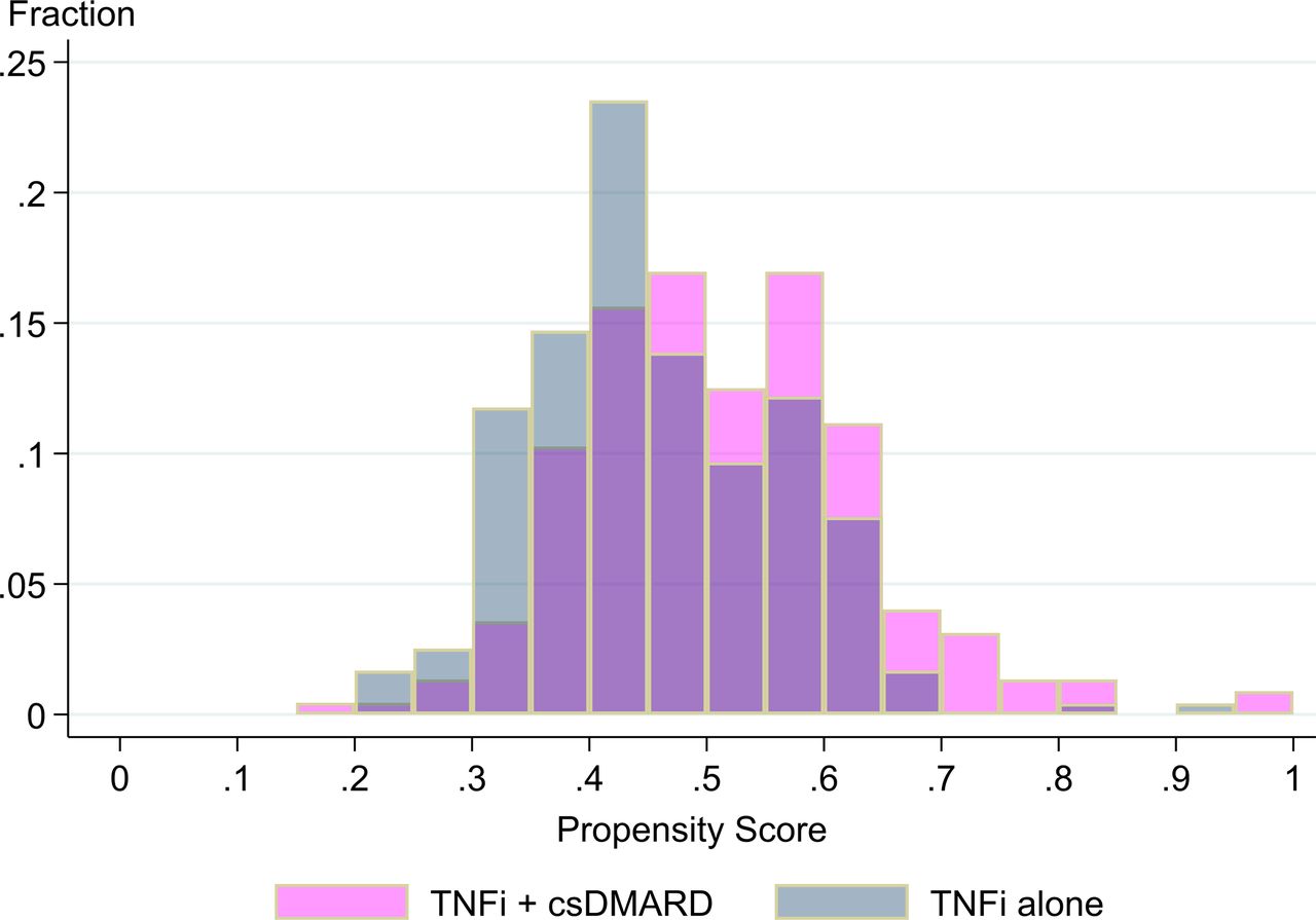
Especially when authors aim for perfect predictability, as in the example above, ‘untied observations’ often occur. These are patients for which we can almost perfectly predict which treatment they will receive. In a proper PS the range of predicted probabilities should cover the entire possible spectrum from 0 to 1, and for each predicted probability a sufficient number of patients that are treated and non-treated should be present.2 One way to think about this is to see PS as an advanced matching technique. It enables us to ‘match’ for many variables at the same time, by compressing those variables into a single score.2 Untied observations are patients without a ‘match,’ which should be deleted. Alternatively, one could trim (ie, delete) patients without a ‘match,’ and patients with a very low probability of receiving one of the treatments. For example, all patients with a PS<0.05.5 When many observations are deleted obviously the data only apply to the resulting selected patient group, which means that the data are less generalisable (figure 1).

• Download figure
• Open in new tab
• Download powerpoint

Figure 1

Propensity score distribution at baseline for two treatment groups. Untied observations fall outside the area of common support (0.20; 0.70) and should therefore be trimmed. Used with permission from Sepriano et al.14 csDMARD, conventional synthetic disease-modifying antirheumatic drug; TNFi, tumour necrosis factor inhibitor.

Two or more than two treatment choices?

Most frequently PS refer to binomial treatment decisions. But in rheumatology there are many scenarios in which multiple treatment options are considered in individual patients. In a previously published study, the clinical outcomes of patients with rheumatoid arthritis (RA) treated according to daily clinical practice were compared after 1 year of treatment in patients who received treatment with either abatacept or tocilizumab.6 The authors describe that in daily practice abatacept and tocilizumab are prescribed to patients with RA with uncontrolled disease despite treatment with conventional synthetic disease-modifying antirheumatic drugs and argue that treatment assignment of either abatacept or tocilizumab may be non-random, that is, different types of patients are being treated with either drug, which will most likely lead to a biased comparison of the outcome. Therefore, they apply PS matching to handle this potential bias.

However, since daily practice data were used, eligible patients could have likely received other treatments than only abatacept or tocilizumab. In theory one could select two of the available treatment options and apply a binomial PS to adjust for confounding by indication (eg, treatments A and B and ignore that patients could also have received C or D). Within the sample of patients starting one of the two selected treatments (ie, A and B), the binomial PS would be valid. However, this would be a gross simplification of the true clinical scenario, in which the rheumatologist had many more treatment options to choose from (ie, C and D). Therefore, external validation falls short, and any generalisation of these data to the whole population of patients with a given disease is not valid. Obviously, this is an important limitation, since one of the main strengths of testing treatment effects with observational data compared with clinical trials is the inclusion of a less selected population, potentially resulting in better generalisability. Therefore, as an alternative, a ‘multiple PS’ should be considered to account for multiple treatment options simultaneously to better reflect reality.7

Step 1: select variables

For the estimation of both binomial and multinomial PS, the first step is the selection of variables to include in the PS. Extensive literature is available regarding variable selection for PS models.4 In short, only variables that are measured before treatment assignment should be included, since variables that are measured after treatment assignment cannot possibly act as confounders (of the treatment allocation process). The highest precision is achieved by adding all variables related to the outcome of the study (eg, disease activity). Variables that are only related to the exposure (eg, treatment), but not to the outcome, decrease precision and should not be included. Ideally, these variables are selected based on subject matter knowledge. However, especially when a large number of pretreatment variables have been collected and the relationship with the outcome is unclear, regression analyses may be used to identify all available pretreatment variables with an association with the outcome. For example, when a continuous measure has been used as outcome, linear regression may be used to select all variables with associations at p<0.10 with the outcome.9

For steps 2–8 a Stata syntax example is available in online supplementary file 1.

Step 2: assess the standardised differences between variables before calculating the PS

This step is not relevant for variable selection or for further analyses, but it provides insight into the initial comparability of the binomial outcome groups by using standardised differences.

Step 3: estimate the PS

Step 4: check the level of balance between treatment and control groups

After obtaining the PS we check the level of balance between treatment and control groups. This can be done by (1) splitting the sample in strata and testing whether the means of the PS are similar within strata across treatment groups (step 5a); and (2) by visual analysis of a density plot of the distribution of the PS in the treatment groups before (figure 1) and after defining the area of common support (step 5b).

Step 4a: check the distribution of the PS in each quintile and per treatment strata

It is common to first split the data in quintiles and investigate the balance across the quintiles. If balance is not achieved, the number of strata can be increased.

Step 4b: find the area of common support

This can be done by creating a histogram similar to figure 1. The area of common support is the range in which the PS for the two groups overlap. The minimum and maximum values defining this range can be used in step 6.

Step 5: graph the PS distribution within the area of common support

Create a similar histogram as in step 4b, but now excluding any data outside the ‘area of common support.’

Step 6: report how many patients were trimmed

Step 7: report the average PS and the number of patients per quintile after trimming

Step 8: assess the standardised differences within quintiles

Standardised difference tests are preferred to examine whether baseline covariates are equally distributed across treatment groups. Standardised differences <0.10 are generally considered acceptable.1

Step 9: re-estimate the PS model if balance is not achieved

Start again with step 3 if balance is not achieved. Options to improve the model include dropping or recategorising variables, or including interaction terms, higher order terms or splines.1 2

Step 10: estimate the effect before applying the PS model

First, perform all analyses without taking the PS into account. This will provide crude results.

Step 11: estimate the effect after applying the PS model

Finally, the PS can be used for matching, stratified sampling, or covariate adjustment in regression analyses. Whereas matching and stratification are performed before doing further statistical analyses, covariate adjustment is incorporated into the analyses. Previous publications are available with a more detailed description of each of these methods for binomial or multiple PS.1 7 9

It has been shown that PS matching is more successful in reducing bias than stratification or covariate adjustment.10–12 However, when multiple exposure groups are compared, matching may not be possible since this may result in small treatment samples.7 9 Furthermore, depending on the planned analyses, covariate adjustment may be considered more appropriate.