Article Text

Abstract
The importance of power and sample size estimation for study design and analysis.
- research design
- sample size
- statistics
Statistics from Altmetric.com
OBJECTIVES
Understand power and sample size estimation.
Understand why power is an important part of both study design and analysis.
Understand the differences between sample size calculations in comparative and diagnostic studies.
Learn how to perform a sample size calculation.
– (a) For continuous data
– (b) For non-continuous data
– (c) For diagnostic tests
POWER AND SAMPLE SIZE ESTIMATION
Power and sample size estimations are measures of how many patients are needed in a study. Nearly all clinical studies entail studying a sample of patients with a particular characteristic rather than the whole population. We then use this sample to draw inferences about the whole population.
In previous articles in the series on statistics published in this journal, statistical inference has been used to determine if the results found are true or possibly due to chance alone. Clearly we can reduce the possibility of our results coming from chance by eliminating bias in the study design using techniques such as randomisation, blinding, etc. However, another factor influences the possibility that our results may be incorrect, the number of patients studied. Intuitively we assume that the greater the proportion of the whole population studied, the closer we will get to true answer for that population. But how many do we need to study in order to get as close as we need to the right answer?
WHAT IS POWER AND WHY DOES IT MATTER
Power and sample size estimations are used by researchers to determine how many subjects are needed to answer the research question (or null hypothesis).
An example is the case of thrombolysis in acute myocardial infarction (AMI). For many years clinicians felt that this treatment would be of benefit given the proposed aetiology of AMI, however successive studies failed to prove the case. It was not until the completion of adequately powered “mega-trials” that the small but important benefit of thrombolysis was proved.
Generally these trials compared thrombolysis with placebo and often had a primary outcome measure of mortality at a certain number of days. The basic hypothesis for the studies may have compared, for example, the day 21 mortality of thrombolysis compared with placebo. There are two hypotheses then that we need to consider:
The null hypothesis is that there is no difference between the treatments in terms of mortality.
The alternative hypothesis is that there is a difference between the treatments in terms of mortality.
In trying to determine whether the two groups are the same (accepting the null hypothesis) or they are different (accepting the alternative hypothesis) we can potentially make two kinds of error. These are called a type I error and a type II error.
A type I error is said to have occurred when we reject the null hypothesis incorrectly (that is, it is true and there is no difference between the two groups) and report a difference between the two groups being studied.
A type II error is said to occur when we accept the null hypothesis incorrectly (that is, it is false and there is a difference between the two groups which is the alternative hypothesis) and report that there is no difference between the two groups.
They can be expressed as a two by two table (table 1⇓).
Two by two table
Power calculations tell us how many patients are required in order to avoid a type I or a type II error.
The term power is commonly used with reference to all sample size estimations in research. Strictly speaking “power” refers to the probability of avoiding a type II error in a comparative study. Sample size estimation is a more encompassing term that looks at more than just the type II error and is applicable to all types of studies. In common parlance the terms are used interchangeably.
WHAT AFFECTS THE POWER OF A STUDY?
There are several factors that can affect the power of a study. These should be considered early on in the development of a study. Some of the factors we have control over, others we do not.
The precision and variance of measurements within any sample
Why might a study not find a difference if there truly is one? For any given result from a sample of patients we can only determine a probability distribution around that value that will suggest where the true population value lies. The best known example of this would be 95% confidence intervals. The size of the confidence interval is inversely proportional to the number of subjects studied. So the more people we study the more precise we can be about where the true population value lies.
Figure 1⇓ shows that for a single measurement, the more subjects studied the narrower the probability distribution becomes. In group 1 the mean is 5 with wide confidence intervals (3–7). By doubling the number of patients studied (but in our example keeping the values the same) the confidence intervals have narrowed (3.5–6.5) giving a more precise estimate of the true population mean.

Change in confidence interval width with increasing numbers of subjects.
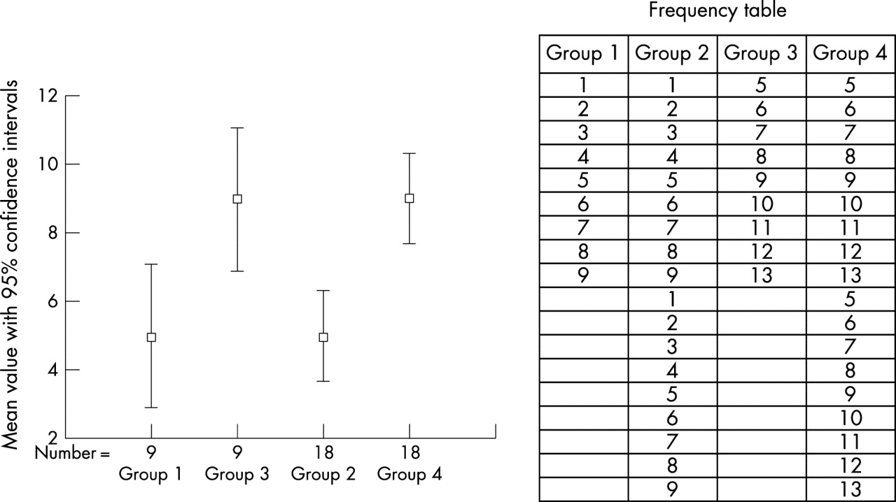
The probability distribution of where the true value lies is an integral part of most statistical tests for comparisons between groups (for example, t tests). A study with a small sample size will have large confidence intervals and will only show up as statistically abnormal if there is a large difference between the two groups. Figure 2⇓ demonstrates how increasing the number of subjects can give a more precise estimate of differences.

Effect of confidence interval reduction to demonstrate a true difference in means. This example shows that the initial comparison between groups 1 and 3 showed no statistical difference as the confidence intervals overlapped. In groups 3 and 4 the number of patients is doubled (although the mean remains the same). We see that the confidence intervals no longer overlap indicating that the difference in means is unlikely to have occurred by chance.
The magnitude of a clinically significant difference
If we are trying to detect very small differences between treatments, very precise estimates of the true population value are required. This is because we need to find the true population value very precisely for each treatment group. Conversely, if we find, or are looking for, a large difference a fairly wide probability distribution may be acceptable.
In other words if we are looking for a big difference between treatments we might be able to accept a wide probability distribution, if we want to detect a small difference we will need great precision and small probability distributions. As the width of probability distributions is largely determined by how many subjects we study it is clear that the difference sought affects sample size calculations.
Factors affecting a power calculation
The precision and variance of measurements within any sample
Magnitude of a clinically significant difference
How certain we want to be to avoid type 1 error
The type of statistical test we are performing
When comparing two or more samples we usually have little control over the size of the effect. However, we need to make sure that the difference is worth detecting. For example, it may be possible to design a study that would demonstrate a reduction in the onset time of local anaesthesia from 60 seconds to 59 seconds, but such a small difference would be of no clinical importance. Conversely a study demonstrating a difference of 60 seconds to 10 minutes clearly would. Stating what the “clinically important difference” is a key component of a sample size calculation.
How important is a type I or type II error for the study in question?
We can specify how concerned we would be to avoid a type I or type II error. A type I error is said to have occurred when we reject the null hypothesis incorrectly. Conventionally we choose a probability of <0.05 for a type I error. This means that if we find a positive result the chances of finding this (or a greater difference) would occur on less than 5% of occasions. This figure, or significance level, is designated as pα and is usually pre-set by us early in the planning of a study, when performing a sample size calculation. By convention, rather than design, we more often than not choose 0.05. The lower the significance level the lower the power, so using 0.01 will reduce our power accordingly.
(To avoid a type I error—that is, if we find a positive result the chances of finding this, or a greater difference, would occur on less than α% of occasions)
A type II error is said to occur when we accept the null hypothesis incorrectly and report that there is no difference between the two groups. If there truly is a difference between the interventions we express the probability of getting a type II error and how likely are we to find it. This figure is referred to as pβ. There is less convention as to the accepted level of pβ, but figures of 0.8–0.9 are common (that is, if a difference truly exists between interventions then we will find it on 80%–90% of occasions.)
The avoidance of a type II error is the essence of power calculations. The power of a study, pβ, is the probability that the study will detect a predetermined difference in measurement between the two groups, if it truly exists, given a pre-set value of pα and a sample size, N.
The type of statistical test we are performing
Sample size calculations indicate how the statistical tests used in the study are likely to perform. Therefore, it is no surprise that the type of test used affects how the sample size is calculated. For example, parametric tests are better at finding differences between groups than non-parametric tests (which is why we often try to convert basic data to normal distributions). Consequently, an analysis reliant upon a non-parametric test (for example, Mann-Whitney U) will need more patients than one based on a parametric test (for example, Student’s t test).
SHOULD SAMPLE SIZE CALCULATIONS BE PERFORMED BEFORE OR AFTER THE STUDY?
The answer is definitely before, occasionally during, and sometimes after.
In designing a study we want to make sure that the work that we do is worthwhile so that we get the correct answer and we get it in the most efficient way. This is so that we can recruit enough patients to give our results adequate power but not too many that we waste time getting more data than we need. Unfortunately, when designing the study we may have to make assumptions about desired effect size and variance within the data.
Interim power calculations are occasionally used when the data used in the original calculation are known to be suspect. They must be used with caution as repeated analysis may lead to a researcher stopping a study as soon as statistical significance is obtained (which may occur by chance at several times during subject recruitment). Once the study is underway analysis of the interim results may be used to perform further power calculations and adjustments made to the sample size accordingly. This may be done to avoid the premature ending of a study, or in the case of life saving, or hazardous therapies, to avoid the prolongation of a study. Interim sample size calculations should only be used when stated in the a priori research method.
When we are assessing results from trials with negative results it is particularly important to question the sample size of the study. It may well be that the study was underpowered and that we have incorrectly accepted the null hypothesis, a type II error. If the study had had more subjects, then a difference may well have been detected. In an ideal world this should never happen because a sample size calculation should appear in the methods section of all papers, reality shows us that this is not the case. As a consumer of research we should be able to estimate the power of a study from the given results.
Retrospective sample size calculation are not covered in this article. Several calculators for retrospective sample size are available on the internet (UCLA power calculators (http://calculators.stat.ucla.edu/powercalc/), Interactive statistical pages (http://www.statistics.com/content/javastat.html).
WHAT TYPE OF STUDY SHOULD HAVE A POWER CALCULATION PERFORMED?
Nearly all quantitative studies can be subjected to a sample size calculation. However, they may be of little value in early exploratory studies where scarce data are available on which to base the calculations (though this may be addressed by performing a pilot study first and using the data from that).
Clearly sample size calculations are a key component of clinical trials as the emphasis in most of these studies is in finding the magnitude of difference between therapies. All clinical trials should have an assessment of sample size.
In other study types sample size estimation should be performed to improve the precision of our final results. For example, the principal outcome measures for many diagnostic studies will be the sensitivity and specificity for a particular test, typically reported with confidence intervals for these values. As with comparative studies, the greater number of patients studied the more likely the sample finding is to reflect the true population value. By performing a sample size calculation for a diagnostic study we can specify the precision with which we would like to report the confidence intervals for the sensitivity and specificity.
As clinical trials and diagnostic studies are likely to form the core of research work in emergency medicine we have concentrated on these in this article.
POWER IN COMPARATIVE TRIALS
Studies reporting continuous normally distributed data
Suppose that Egbert Everard had become involved in a clinical trial involving hypertensive patients. A new antihypertensive drug, Jabba Juice, was being compared with bendrofluazide as a new first line treatment for hypertension (table 2⇓).
Egbert writes down some things that he thinks are important for the calculation
As you can see the figures for pα and pβ are somewhat typical. These are usually set by convention, rather than changing between one study and another, although as we see below they can change.
A key requirement is the “clinically important difference” we want to detect between the treatment groups. As discussed above this needs to be a difference that is clinically important as, if it is very small, it may not be worth knowing about.
Another figure that we require to know is the standard deviation of the variable within the study population. Blood pressure measurements are a form of normally distributed continuous data and as such will have standard deviation, which Egbert has found from other studies looking at similar groups of people.
Once we know these last two figures we can work out the standardised difference and then use a table to give us an idea of the number of patients required.

The difference between the means is the clinically important difference—that is, it represents the difference between the mean blood pressure of the bendrofluazide group and the mean blood pressure of the new treatment group.
From Egbert’s scribblings:

Using table 3⇓ we can see that with a standardised difference of 0.5 and a power level (pβ) of 0.8 the number of patients required is 64. This table is for a one tailed hypothesis, (?) the null hypothesis requires the study to be powerful enough to detect either treatment being better or worse than the other, so we will need a minimum of 64×2=128 patients. This is so that we make sure we get patients that fall both sides of the mean difference we have set.
How power changes with standardised difference
Another method of setting the sample size is to use the nomogram developed by Gore and Altman2 as shown in figure 3⇓.

Nomogram for the calculation of sample size.
From this we can use a straight edge to join the standardised difference to the power required for the study. Where the edge crosses the middle variable gives an indication as to the number, N, required.
The nomogram can also be used to calculate power for a two tailed hypothesis comparison of a continuous measurement with the same number of patients in each group.
If the data are not normally distributed the nomogram is unreliable and formal statistical help should be sought.
Studies reporting categorical data
Suppose that Egbert Everard, in his constant quest to improve care for his patients suffering from myocardial infarction, had been persuaded by a pharmaceutical representative to help conduct a study into the new post-thrombolysis drug, Jedi Flow. He knew from previous studies that large numbers would be needed so performed a sample size calculation to determine just how daunting the task would be (table 4⇓).
Sample size calculation
Once again the figures for pα and pβ are standard, and we have set the level for a clinically important difference.
Unlike continuous data, the sample size calculation for categorical data is based on proportions. However, similar to continuous data we still need to calculate a standardised difference. This enables us to use the nomogram to work out how many patients are needed.
p1=proportional mortality in thrombolysis group =12% or 0.12

p2=proportional mortality in Jedi Flow group =9% or 0.09 (This is the 3% clinically important difference in mortality we want to show).
P=(p1+ p2)/2=


The standardised difference is 0.1. If we use the nomogram, and draw a line from 0.1 to the power axis at 0.8, we can see from the intersect with the central axis, at 0.05 pα level, we need 3000 patients in the study. This means we need 1500 patients in the Jedi Flow group and 1500 in the thrombolysis group.
POWER IN DIAGNOSTIC TESTS
Power calculations are rarely reported in diagnostic studies and in our experience few people are aware of them. They are of particular relevance to emergency medicine practice because of the nature of our work. The methods described here are taken from the work by Buderer.3
Dr Egbert Everard decides that the diagnosis of ankle fractures may be improved by the use of a new hand held ultrasound device in the emergency department at Death Star General. The DefRay device is used to examine the ankle and gives a read out of whether the ankle is fractured or not. Dr Everard thinks this new device may reduce the need for patients having to wait hours in the radiology department thereby avoiding all the ear ache from patients when they come back. He thinks that the DefRay may be used as a screening tool, only those patients with a positive DefRay test would be sent to the radiology department to demonstrate the exact nature of the injury.
He designs a diagnostic study where all patients with suspected ankle fracture are examined in the emergency department using the DefRay. This result is recorded and then the patients are sent around for a radiograph regardless of the result of the DefRay test. Dr Everard and a colleague will then compare the results of the DefRay against the standard radiograph.
Missed ankle fractures cost Dr Everard’s department a lot of money in the past year and so it is very important that the DefRay performs well if it be accepted as a screening test. Egbert wonders how many patients he will need. He writes down some notes (table 5⇓).
Everard’s calculations
For a diagnostic study we calculate the power required to achieve either an adequate sensitivity or an adequate specificity. The calculations work around the standard two by two way of reporting diagnostic data as shown in table 6⇓.
Two by two reporting table for diagnostic tests
To calculate the need for adequate sensitivity


To calculate the need for adequate specificity
If Egbert were equally interested in having a test with a specificity and sensitivity we would take the greater of the two, but he is not. He is most interested in making sure the test has a high sensitivity to rule out ankle fractures. He therefore takes the figure for sensitivity, 243 patients.


CONCLUSION
Sample size estimation is key in performing effective comparative studies. An understanding of the concepts of power, sample size, and type I and II errors will help the researcher and the critical reader of the medical literature.
QUIZ
What factors affect a power calculation for a trial of therapy?
Dr Egbert Everard wants to test a new blood test (Sithtastic) for the diagnosis of the dark side gene. He wants the test to have a sensitivity of at least 70% and a specificity of 90% with 5% confidence levels. Disease prevalence in this population is 10%.
– (i) How many patients does Egbert need to be 95% sure his test is more than 70% sensitive?
– (ii) How many patients does Egbert need to be 95% sure that his test is more than 90% specific?
If Dr Everard was to trial a new treatment for light sabre burns that was hoped would reduce mortality from 55% to 45%. He sets the pα to 0.05 and pβ to 0.99 but finds that he needs lots of patients, so to make his life easier he changes the power to 0.80.
How many patients in each group did he need with the pα to 0.05 and pβ to 0.80?
How many patients did he need with the higher (original) power?
Quiz answers
See box.
(i) 2881 patients; (ii) 81 patients
(i) about 400 patients in each group; (ii) about 900 patients in each group
Acknowledgments
We would like to thank Fiona Lecky, honorary senior lecturer in emergency medicine, Hope Hospital, Salford for her help in the preparation of this paper.
Footnotes
Correction notice Following recent feedback from a reader, the authors have corrected this article. The original version of this paper stated that: “Strictly speaking, “power” refers to the number of patients required to avoid a type II error in a comparative study.” However, the formal definition of “power” is that it is the probability of avoiding a type II error (rejecting the alternative hypothesis when it is true), rather than a reference to the number of patients. Power is, however, related to sample size as power increases as the number of patients in the study increases. This statement has therefore been corrected to: “Strictly speaking, “power” refers to the probability of avoiding a type II error in a comparative study.
Linked Articles
- Correction
- Correction