The nested case-control design is an efficient approach for investigating exposure-disease associations in a study population.¹ This approach is particularly useful in studies of large cohorts, since the time and cost involved in collecting exposure and covariate information for all members of a large study cohort may be substantial. By drawing a sample of controls for each case, the number of study subjects for whom exposure information needs to be obtained is reduced. The nested case-control design is also useful as a method for computational reduction, which is achieved by drawing a sample of the eligible controls and organising the study data in a form for analysis by conditional logistic regression.

While various methods have been used for sampling controls in nested case-control analyses, incidence density sampling is the method of choice for obtaining unbiased results.² An efficient incidence density sampling scheme is one in which controls are selected without replacement from all persons at risk at the time of case occurrence, excluding the index case itself.³

Two programs for incidence density sampling have been described previously in the epidemiological literature. Beaumont et al described a system for incidence density sampling developed by the National Institute for Occupational Safety and Health (NIOSH).⁴ The NIOSH system encompasses a series of programs written to operate in the IBM mainframe environment. Controls are matched to cases on attained age, with the option of additional matching on sex, race, year of birth, and duration of employment. Pearce proposed a simpler program that could be run a personal computer and easily accommodate an investigator’s choice of matching variables.⁵ While the program proposed by Pearce has the advantages of being easy to implement on a personal computer and flexible in accommodating an investigator’s needs, it is essentially a modified program for person-time tabulation and consequently suffers some limitations. Since an observation is created for each unit of follow up time (for example, person-year), the program is best suited to approximate matching of controls to cases on a timescale such as attained age, rather than exact matching on that timescale. Furthermore, in a tabulation of person-time, an individual contributes a single observation for each unit of follow up regardless of the number of cases that arise during that time interval; in contrast, in incidence density sampling, a person is eligible to serve as a control for multiple cases at a given moment in time. Pearce’s program does not allow for this possibility.

This paper presents a simple program for incidence density sampling. This program is evaluated using empirical data for a large occupational cohort.

METHODS

In incidence density sampling, controls are selected from among those persons under study who survived at least as long as the index case. Survival may be defined in terms of attained age, time since treatment, or some other timescale. Attained age is often the timescale of interest since disease rates typically are strongly associated with age; creating risk sets that are matched on attained age achieves perfect control for potential confounding by this factor.⁶

Table 1 describes the basic cohort data needed to select controls by incidence density sampling on attained age using the Statistical Analysis System (SAS) program shown in the Appendix.⁷ The requirements are simple enough to apply to a variety of epidemiological studies in which a cohort is enumerated and followed over time to identify incident disease or mortality.

Four variables are required on the source file used by the program. The variable age_entry indicates a person’s age, in days, at entry in the study. The variable age_dlo indicates a person’s age, in days, at last observation (that is, case occurrence, censoring, or end of study). The variable censor is a binary indicator of case status; and the variable study_id is a unique numeric study identifier.

In the first two lines of the program the user specifies whether sampling of controls will occur, and, if so, the ratio of controls to cases. The variable sampling may be assigned a value of “yes” or “no”. If “no” is specified then each index case is matched to all eligible controls. If “yes” is specified then a specified number of controls are randomly selected for each case from the pool of all eligible controls; the variable ratio specifies the number of controls to select per case.

Next, the number of cases in the study cohort is enumerated. The number of cases in the study cohort is equal to the number of risk sets that need to be created by incidence density sampling. For each case, the age at time of failure for the index case is identified and denoted, age_rs. A temporary data set is constructed of all eligible controls for the index case. The pool of eligible controls includes all cohort members (with the exception of the index case itself), whose age at entry into the study was less than or equal to the attained age of the index case and whose age at end of study was greater than or equal to the attained age of the index case. Controls may be drawn by random sampling from this pool of eligible controls to form the incidence density sampled risk set for the index case. These risk sets, indexed by the variable rs, are appended together to generate the final analytical data set, final.

Covariate information that is fixed (for example, sex, race) may be retained as additional variables associated with each observation output to a risk set. Covariate information that is time dependent (for example, cumulative exposure level) can be calculated after the risk sets are created by reference to the exact date that each person in a risk set reached the attained age of the index case (that is, age_rs days after the person’s date of birth).

An investigator may wish to control for potential confounding by matching on one or more covariates (rather than modelling the covariate effects). Incidence density sampling with matching on a covariate (for example, sex) is easily accommodated by this program (see http://www.unc.edu/~davidr/id). Matching on a covariate when selecting controls via incidence density sampling will lead to conditional logistic regression estimates of association that approximate those obtained in a Cox proportional hazards regression analysis that is stratified on that covariate.

Pearce’s incidence density program

The algorithm for incidence density sampling that Pearce proposed is an adaptation of a program for generating person-time data.^5,8 Pearce’s incidence density sampling program generates a data set that has a unique observation for each unit of person-time; person-time may be partitioned into units of person-years or into smaller units (for example, person-months or person-days). An individual contributes observations to the pool of eligible controls through the penultimate unit of person-time. The observation for the final unit of follow up time, however, does not contribute to the pool of eligible controls (for any case); it is solely a case record.

There are several limitations to the program proposed by Pearce.⁵ Firstly, regardless of whether person-time is partitioned into units of person-years or person-days, the attained age of each case is rounded down to the nearest year (the case’s age on their last birthday). Consequently, risk sets are not matched exactly on age, and therefore time dependent covariates may not be correctly specified. For example, calendar year at risk (or cumulative exposure level) assigned to a control based on the birthday when they reach the age of the case is not necessarily the same value that would be assigned to that control if matching were done according to the exact age of the case.

Secondly, a case is excluded from all risk sets enumerated during the time interval spanned by their final period (for example, person-year) of follow up. Therefore, the pool of controls for a given case does not include any other case that attained that age in their final period of follow up.

Thirdly, a control is excluded from serving in more than one risk set that is enumerated at a given year of age. If multiple cases occur at a given year of age, a person who is eligible to serve as a control can be selected for only one of the cases. For example, if five cases occur at 76 years of age, then a person who is alive and under study at age 76 should be eligible to serve as a control for each of these cases. However, under Pearce’s program, the person who is alive and under study at age 76 may serve as a control for only one of these cases. Since the attained age of each case is rounded downward to the nearest year (that is, the case’s age on their last birthday), multiple cases may occur at the same age.

Finally, under Pearce’s program, a case may be selected to serve as its own control. Again, this occurs because the attained age of each case is rounded down to the nearest year, so the case may have contributed a unit of person-time at risk to the pool of controls for the period spanning their last birthday. Consequently, if follow up time is partitioned into units smaller than a person-year then the pool of controls for a given case may include the case itself.

In order to illustrate the differences between the incidence density sampling program proposed in this paper and the program proposed previously by Pearce,⁵ a hypothetical cohort that included eight people (and three cases) was constructed. Using these data, incidence density sampling was used to construct a nested case-control study with three controls per case, and a nested case-control study with four controls per case. Incidence density sampling was performed using the program shown in the Appendix and using the program proposed by Pearce (1989). The risk sets enumerated by each approach were compared (see http://www.unc.edu/~davidr/id).

Statistical methods

In order to illustrate the consequences of the differences between these incidence sampling algorithms for epidemiological risk estimates, nested case-control analyses were conducted using data for a cohort of 8307 white males hired from 1943 and 1972 who worked at least 30 days at Oak Ridge National Laboratory (ORNL).⁹ Vital status through 1990 was ascertained through Social Security Administration, National Death Index, and employer records. At the close of follow up, 5879 (70.8%) members of the cohort were still alive, 2110 (25.4%) members had died, and 318 (3.8%) members had been lost to follow up. The exposure variable of interest in these analyses is pay code, which has been used previously as an indicator of socioeconomic status and shown to be an important predictor of mortality risk.^10,11 For these analyses, a fixed dichotomous variable was defined by the worker’s pay code at date of hire; a comparison was drawn between weekly paid workers and other workers.

Controls were selected for cases by incidence density sampling using the program presented in the Appendix of this paper. Conditional logistic regression, via SAS PROC PHREG, was used to derive an estimate of the pay code-mortality association, .^7,12 The regression model included a single parameter for pay code, with attained age exactly controlled for via stratification. The process of selecting controls and deriving an estimate of the exposure-mortality association was repeated over 100 iterations after which the average effect estimate, , was calculated.

Cox proportional hazards regression, via SAS PROC PHREG, was used to derive an estimate of the pay code-mortality association, , using data for the full cohort.^7,12 The proportional hazards regression model also included a single parameter for pay code, with attained age as the time scale. The ratio of to is referred to as bias; a value of unity indicates that results obtained via conditional logistic regression analyses of nested case-control data, on average, equal the result obtained via Cox proportional hazards regression.

These analyses were repeated under sampling ratios (number of controls per case) of 10:1, 50:1, and 100:1. The same methods were used to evaluate the incidence density sampling program proposed by Pearce⁵ with follow up time tabulated in units of person-years and in units of person-months.

RESULTS

Analyses were first conducted using the incidence density sampling program shown in the Appendix (method I). The estimate of the relative risk of all cause mortality when comparing weekly paid workers to other workers was derived via conditional logistic regression analyses of nested case-control data. Ten controls were selected for each case. After 100 iterations of this procedure, the average effect estimate () approximated the result obtained via proportional hazards regression using data for the full cohort ().

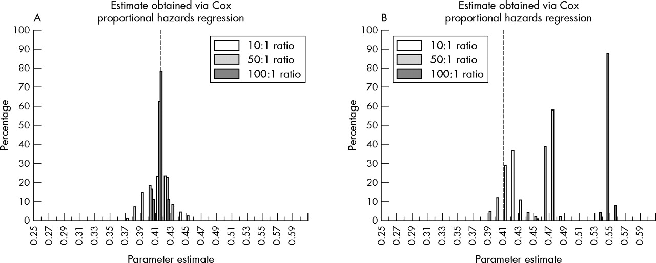
Table 2 reports the approximate bias in the average parameter estimate derived via conditional logistic regression after 100 repetitions of nested case-control analyses with 10, 50, and 100 controls per case. A value of unity indicates an absence of bias in conditional logistic regression results (relative to the estimate obtained via proportional hazards regression). For analyses conducted using the incidence density sampling method I, values for this coefficient of bias were equal to unity under each of the sampling ratios evaluated. Figure 1A presents a histogram of the conditional logistic regression parameter estimates obtained from 100 nested case-control analyses conducted with 10, 50, and 100 controls per case. Estimates of association are distributed relatively symmetrically around the value of the parameter estimate obtained via proportional hazards regression.

Table 2 also presents coefficients of bias for conditional logistic regression estimates obtained from nested case-control analyses with incidence density sampling performed using the program proposed by Pearce (method II). For analyses in which 10 controls were selected per case, there was little of evidence of bias in the average effect estimate obtained via conditional logistic regression (relative to the estimate obtained via proportional hazards regression). In contrast, for analyses in which 50 or 100 controls were selected for each case, there was clear evidence that the resultant parameter estimates were positively biased. Figure 1B presents a histogram of the conditional logistic regression parameter estimates obtained from 100 nested case-control analyses conducted with 10, 50, and 100 controls per case. With incidence density sampling conducted using method II, the resultant estimates of association are progressively skewed away from the value for the parameter estimate obtained via proportional hazards regression as the sampling ratio increases.

We repeated the analyses in table 2 with incidence density sampling performed using Pearce’s program with person-time partitioned into units of person-months (rather than person-years). Results were similar to those reported in table 2; average coefficients of bias for conditional logistic regression parameter estimates obtained from 100 nested case-control analyses conducted with 10, 50, and 100 controls per case were 1.01, 1.09, and 1.25, respectively.

DISCUSSION

A case-control study nested within a cohort can be a highly efficient method for epidemiological investigation. If exposure data are costly or difficult to collect, then use of a nested case-control approach may facilitate an investigation by reducing the number of subjects for whom exposure data are needed. However, even when exposure data are available for all cohort members, analysis of cohort data via the nested case-control approach offers a useful method for computational reduction when compared to Cox regression.¹ In Cox proportional hazards regression, the risk set for an incident case includes all persons at risk at the moment instantaneously prior to case occurrence (therefore including the case itself). Incidence density sampling is a method of forming a sub-sample of that risk set. The index case is matched to a specified number of controls drawn from the full risk set. The index case—and only the index case—should be excluded from the pool of eligible controls if sampling of controls is done without replacement.³

These considerations are directly relevant to understanding the bias observed in analyses (table 2) when incidence density sampling was performed using the program proposed by Pearce.⁵ Bias arose as a result of the inappropriate exclusion of subjects from the pool of eligible controls. Under the incidence density sampling program proposed by Pearce, a case is excluded from all risk sets enumerated during the time interval spanned by their final period (for example, person-year) of follow up. Also, under the incidence density sampling program proposed by Pearce, if multiple cases arise at a given year of age, a person is excluded from serving as a control for more than one of the cases. The inappropriate enumeration of risk sets when using the incidence density sampling program proposed by Pearce can be illustrated by means of a simple example using hypothetical cohort data (see http://www.unc.edu/~davidr/id).

The analyses of empirical data (table 2) suggest that the degree of bias arising due to these problems with the incidence density sampling program proposed by Pearce may be minimal if the number of controls selected per case is small relative to the total size of the risk set. In situations where a nested case-control study design is used to reduce the cost and time involved in data collection, it is unusual to select more than 10 controls per case. However, incidence density sampling is also used as a means of computational reduction. Cox proportional hazards regression is a standard approach to analyses of continuous cohort data, but conditional logistic regression with incidence density sampling offers an efficient alternative to Cox regression analyses. When using the latter approach, an investigator may select a relatively large number of controls for each case (for example, 50 or more) in order to preserve the precision of risk estimates while still benefiting from the computational efficiency afforded by incidence density sampling. The analyses in this paper suggest that under these conditions, the program proposed by Pearce may lead to highly biased risk estimates (while the program reported in the Appendix will produce unbiased risk estimates). In the example presented in table 2, the direction of bias was away from the null; however, inflation, attenuation, or reversal of exposure-disease associations would be possible as a result of the problems in the incidence density sampling program proposed by Pearce.

Given the advances in the processing speed of personal computers, exact incidence density sampling can be achieved via this relatively simple program. This approach allows an investigator to take advantage of the efficiencies associated with the nested case-control design without producing biased risk estimates.

APPENDIX

SAS program for incidence density sampling

%macro caseset;

%let sampling = ‘yes’;

%let ratio = 10;

** Enumerate Cases **;

data cases;

set source ;

if censor = 1;

run;

data cases;

set cases end = eof;

if eof then call symput (‘ncases’, put(_n_,6.));

run;

** Create Risk Set **;

%do iter  =  1 %to &ncases;

data temp_case;

set cases;

if _n_  = &iter ;

call symput (‘rs’, put(_n_,6.));

call symput (‘age_rs’, put(age_dlo,8.)); call symput (‘case_id’, put(study_id,8.));

run;

data temp_control;

set source;

if age_entry < =  &age_rs < = age_dlo;

** Exclude Index Case **;

if study_id = &case_id then delete;

number = ranuni(0);

age_rs = &age_rs;

censor = 0;

run;

**Sample Controls **;

%if &sampling = ‘yes’ %then %do;

proc sort data = temp_control;

by number;

data temp_control;

set temp_control;

by age_rs;

retain m;

if first.age_rs then m = 0;

m = m+1;

if m< = &ratio then output temp_control;

run;

%end; * End If Sampling = yes;

** Combine Case with Controls **;

data rs_&iter;

set temp_case

temp_control;

rs = &rs;

age_rs = &age_rs;

run;

DM “Output; Clear; Log; Clear”;

%end; * End Loop Creating Risk Set;

** Append Risk Sets **;

%do j  =  2 %to &ncases;

proc append base  =  rs_1 data  =  rs_&j;

run;

%end;

data final; set rs_1; run;

%mend ; ** End Macro **;

** Invoke Macro **;

%caseset;