METHODS

Introductory issues

To set the stage for the presentation of the novel and most complex model, the basic ideas behind the relative survival approach are first reviewed. The three alternative models, which are simpler and to some extent special cases of each other, should then need little elaboration. The formal specification of all models is followed by a brief description of data and an account of some technical details. For pedagogical purposes, the differences between the models are illustrated in a graph.

A piecewise constant mortality rate is assumed in all models. With such specification, one can generally get a better fit to the duration pattern than with the less flexible parametric models. Besides, models with piecewise constant rates and categorical covariates are convenient to estimate, and are, in fact, indistinguishable from Poisson regression (of number of deaths with exposure time as “offset”, that is, conditional on exposure time).¹² This means that one can make use of the Poisson regression module in Epicure, which has the special advantage that it permits the partly additive structure needed for the relative survival approach.

The rationale for the relative-survival approach

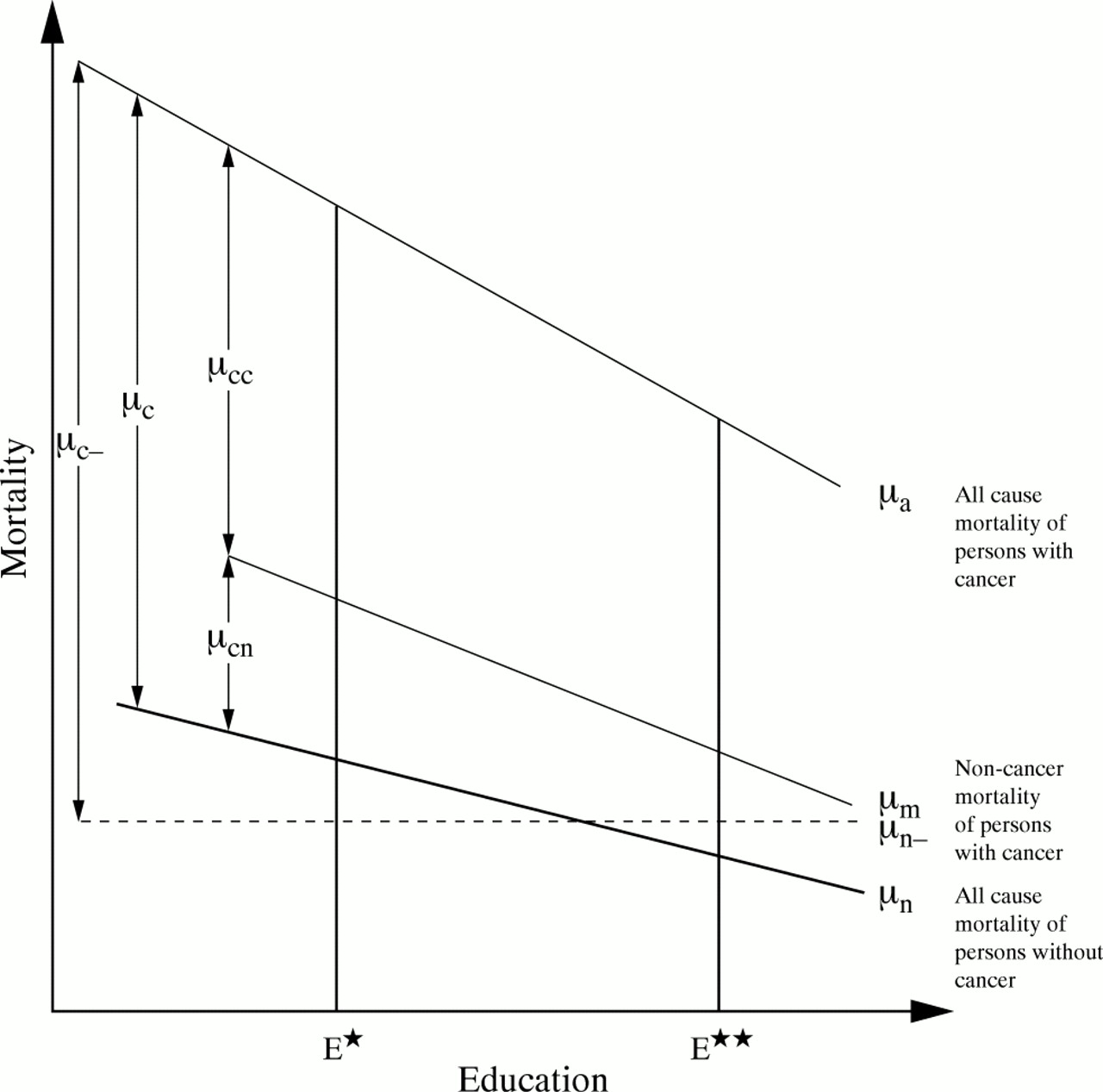
The idea behind the relative-survival approach is illustrated in figure 1, which is drawn for a given age, sex, and period. The bold line is mortality for persons without a cancer diagnosis (μ_n). It is depicted, for simplicity, as declining linearly with educational level, but that is of no importance for the argument that follows. According to Norwegian regulations, cancer can never be the formal cause of death among this group.

Among those who have received a cancer diagnosis, death is, of course, very often registered as the result of cancer. This “registered cancer mortality” is denoted here as μ_cc, while the cancer patients' all cause mortality is μ_a. In addition, it is likely that persons with a cancer diagnosis may suffer an extra high non-cancer mortality as a result of their disease—that is, that their mortality from other registered causes (μ_m) is higher than that among other persons (μ_n). To give just one example, the emotional stress from cancer may increase the chance of being involved in a motor vehicle accident, which may then (correctly) be registered as the cause of death.

Because of this blurredness of the cause of death, and because cause specific mortality data are not always available, “relative survival” was suggested several decades ago as a fruitful measure of the aggressiveness of the disease. It is defined as the ratio of (all cause) survival for cancer patients within, say, a five year interval to that among persons without such a diagnosis, and corresponds to the sum μ_c of μ_cc and μ_cn. (When mortality of a cancer patient is μ=μ_a=μ_n+μ_c and that of another person is μ=μ_n , relative survival can be found by exponentiating the negative integral of μ_c over the relevant duration interval. Mathematically, five year relative survival is R₅ = exp(- ∫ μ_a dw)/ exp(- ∫ μ_n dw) = exp(- ∫ μ_c dw), where the integration is over duration w=0 to w=5 years.)

The novel approach: an extended CS version of the relative survival approach (model 1a)

The extended CS version is specified as

where μ is all cause mortality and x is a vector of categorical sociodemographic variables (covariates), such as age, period, educational level, and marital status. b and c are effect vectors, and y is a cancer diagnosis indicator that takes the value 1 from the time of diagnosis (if any) of the cancer under investigation, and otherwise is 0. The covariate vector z includes various characteristics of the disease, and d is the corresponding effect vector.

For a person without the cancer in focus (that is, y=0), and with sociodemographic characteristics x, mortality is e ^{b x}. This is, of course, the multiplicative structure we usually see in hazard models, and it means that mortality is a product of various positive factors. This first additive term, e^bx, is referred to in this study as “normal” mortality. It is close to, but not exactly equal to, the national mortality level, as people with this particular cancer, which is a quite small group, are left out. The second term, e ^{c x} e ^{d z} , is always positive and is the excess mortality of otherwise similar persons who have been diagnosed with this particular type of cancer.

The three simpler models used in previous studies

Model 1b: the simple CS version of the relative survival approach

The inclusion of only age, sex, and period in the first term, and not education or marital status, can be symbolised by a different covariate x- in the equation, which thus looks like:

This means that “normal” mortality (given age, sex, and period) is assumed to be a constant line μ_n- rather than a varying μ_n.

This model is essentially the same as the simple HT version of the relative survival approach, except that “normal” mortality is modelled, rather than taken as constants.

Model 2a: observed survival

The simplest approach is to model all cause mortality for a sample of cancer patients exclusively. This model can be written as

Model 2b: cause specific survival

Alternatively, one may estimate cancer patients' risk of dying from cancer, according to the “main cause” of death recorded on the death certificates. The model thus becomes

In the Norwegian data, a large majority of those who die within five years of diagnosis are reported as dying from the malignant disease. The proportion is 70%–95%, depending on the cancer site, with 90% as an average.

Data

The analysis is based on individual sociodemographic biographies for all men and women with a Norwegian identification number (that is, all those who have lived in Norway for some time after 1960). These life histories have been extracted from the Norwegian Population Register, the Cause of Mortality Register and the Population Censuses of 1960, 1970, and 1980, and include information about date and cause of death and all changes in residence, as well as marital status, education, income and occupation at the time of the censuses. They have been linked with data from the Norwegian Cancer Registry, which from 1953 has received information on all cancer cases in the population (site, basis for the diagnosis, histological grade and type, and the stage of the disease at the time of diagnosis). These linked data have been used in several previous studies.^1,2,10,11,13

Twelve common cancer sites are considered in the analysis. At ages 40–80 during the observation period 1960–1991, there were more than 150 000 deaths among men or women diagnosed with cancer less than five years previously. Three quarters of these deaths were among persons with cancer in one of the 12 selected sites.

Detailed specifications

In all these models, the men and women are followed up from age 50 (or 40 in models for leukaemia, malignant melanoma, and cancer in the breast or female genitals, which tend to occur at a lower age) or, if born before 1910 (or 1920), from 1960. It is censored at age 80 (because of potentially inadequate case ascertainment at higher ages), at the time or emigration, or by the end of 1991, which was the end of the follow up period. Moreover, people are excluded from the analysis (that is, contribute neither exposure nor deaths) during periods when they lived in another country. In addition, those who did not participate in one of the censuses are excluded during the 10 years after this census. These two restrictions have very little influence on total exposure time. The very few persons with a cancer diagnosed at necropsy are treated as having never received a cancer diagnosis. (Estimated survival gradients might be slightly affected, because of possible sociodemographic differentials in the diagnostic intensity or necropsy frequency, but this should be of no concern when the focus is on differences between models).

Some cancer types may cause death already after a few months, while others may be relatively harmless for many years, perhaps followed by recurrences. In this study, the observations are censored five years after diagnosis, if any. This interval is commonly used in cancer survival analysis. The model thus provides information on how the various sociodemographic variables influence excess mortality “on the whole” over the five years after diagnosis. (A more detailed picture could have been established by including interactions with duration since diagnosis, or by estimating additional models for other interval lengths.)

Mortality is assumed to be constant within five year age groups, which was experimentally found to be a sufficient control for age.

There is no distinction between persons who had previously been diagnosed with another type of cancer and those for whom the cancer in focus was the first one.

All covariates are categorical. They are also time varying: a level for the covariate is defined for each month during the follow up period, and refers to the situation at that time (age, period) or that in the last previous census (education and marital status).

The z-vector includes subsite, stage, and histological type and/or grade, whenever relevant. Stage is defined as localised, regional spread, distant spread, or unknown. The categorisation of histology and subsite differs across cancer sites and is explained in notes to table 2. The intention behind the categorisation is to distinguish at least between quite large histological groups or subsites associated with markedly different survival rates.

In addition, a few models that are not site specific are estimated. A site variable is then included in z, and (for the models 1a and 1b) y takes the value 1 from the time of diagnosis of any of the 12 cancers. Only the first cancer diagnosis is considered in this set up.

The models are estimated in the Amfit Poisson regression module in the Epicure software.¹⁴ A self made computer program (written in Pascal), operating on the individual level register and census data, was used to compute the tables of deaths and exposures that were fed into Amfit. For each person and each month of follow up, a contribution of one month was added in the appropriate cell of the exposure table (defined according to the level of each covariate at that time). One death was added to the table of deaths, in the appropriate cell, if follow up was ended by death.

RESULTS

Education effects estimated from the model that permits educational variations in “normal” mortality

For pedagogical purposes, all estimates from model 1a, including those for variations in “normal” mortality, are shown for one cancer site. Colorectal cancer has been chosen (table 1). Men in the arbitrarily chosen reference category (that is, aged 65–69, observed 1960–69, compulsory education) have a “normal” mortality of 0.0025 deaths per person month. Otherwise similar men who have a post-secondary education at a low level have a “normal” mortality that is 25% lower, while it is 36% lower for the few who have reached a level corresponding to a master's degree. (The corresponding figures for women are almost the same; not shown).

Turning now to the second term, it is found that men in the reference category who have a localised, well differentiated adenocarcinoma in caecum or ascendence (which is the reference category for the disease variable) experience 0.0051 deaths per person month more than otherwise similar men without this disease. For those who have an education at a master's level, but are otherwise similar, the corresponding excess mortality is 17% lower than this. The excess mortality declines monotonically with education.

The estimated effects of educational level on excess mortality from colorectal cancer in men are shown also in table 2, along with corresponding estimates from other cancer sites and for women. The figures at the bottom of the table are for all the 12 cancer sites pooled.

Education effects estimated from other models

In table 3, the estimates shown in table 2 are compared with those from the three other models. For simplicity, men or women with only compulsory education, which are the reference group, are excluded from this table. (To facilitate the reading of the table, differences of 0.03–0.05 are shown in bold types and those larger than 0.05 in underlined bold types.)

When “normal” mortality is assumed to be independent of education (model 1b), the excess mortality of those with secondary or higher education compared with those with only a compulsory education becomes smaller. In other words, the effects of education on survival become sharper.

The differences are minor for some malignancies, such as lung cancer, pancreas cancer and stomach cancer, but are quite large for prostate cancer, bladder cancer and malignant melanoma. According to model 1b, men with an education at the master's level would have an excess mortality from prostate cancer that is 44% lower than that among men with only compulsory education. However, when it is taken into account that they would have had a much lower mortality also in the absence of the disease (model 1a), this advantage is reduced to 34%. The corresponding figures for men with one to four years of secondary education are 11% and 4%.

Because the control for educational differentials in “normal” mortality has little impact for most of the cancer sites, the differences between models 1a and 1b are rather small when all sites are pooled. They range from 0.02 to 0.05.

While the exclusion of education from the first term of the model reduces the estimated excess mortality relative to the reference category (that is, gives an exaggerated impression of the importance of educational level for survival), there is a further change in the opposite direction when the term is entirely removed (model 2a). With only quite few exceptions, the estimates are closer to 1 than those obtained from model 1b, and thus also nearer those from model 1a.

If only the deaths reported as attributable to the cancers in focus are counted (model 2b), the effects of education are, on the whole, slightly weaker. When all cancer sites are pooled, the differences between model 2a and model 2b are 0.01–0.03.

Marital status effects

Similar patterns appear when marital status is considered instead of education. The effects of marital status on excess mortality from different types of cancer, according to the most complex model (1a), are shown in table 4.

The differences in “normal” mortality are even larger for marital status than for education. Never married men have a 30% higher `normal' mortality than the married, while that of widowers is 25% higher and that of the divorced 79% higher (not shown). The corresponding figures for women are lower.

Divorced men are found to have an excess mortality from prostate cancer that is 45% higher than that of married men, according to model 1b, but when their much higher mortality in the absence of the disease is taken into account (model 1a), this difference is reduced to 23% (table 5). Similarly, the relatively high excess mortality for widowers completely disappears, and that for never married is almost halved, from 24% to 14%.

Quite large differences between models are found also for colorectal cancer, bladder cancer, and malignant melanoma. The differences between models 1b and 2a are as explained above for models including educational level: by and large, estimates from model 2a are nearer 1 and nearer those from model 1a.

If registered cancer mortality is modelled instead (model 2b), the effects are, on the whole, slightly weaker than those from model 2a. When all cancer sites are pooled, the differences between model 2a and model 2b for divorcees are 0.03–0.04. The differences are smaller for the never married and widowed.

DISCUSSION

A view to the Hakulinen-Tenkanen version

In the HT version of the relative survival approach, “normal” mortality (or, rather, survival) rates are defined for relevant subgroups, for example all possible combinations of age, sex, and period, and considered as constants. A ratio between patient survival and “normal” (often denoted as “expected”) survival is calculated for each covariate combination (cell). Using a log-log transformation of this ratio, which yields a linear structure of sociodemographic (and other) effects, the estimation is easily carried out in the GLIM software.

In the extended version of this,⁹ social-status-specific “normal” mortality rates were first calculated from individual data (but, as explained in the paper, they could also have been taken from published life tables adjusted by social status correction factors derived from other sources). However, if such individual data exist, and can be linked with data on cancer diagnosis, also model 1a presented here can be estimated. Model 1a should in some respects be slightly more satisfying, without necessarily giving perceptibly different results.

Firstly, “normal” mortality is not treated as a constant. When data for a large national population are used to establish “normal” mortality, it is, of course, acceptable to use only point estimates for each cell and disregard information on variance. This is less satisfying when one has access only to a smaller sample (perhaps supposed to be representative of the national population). When variances in “normal” mortality are no longer negligible compared with the variances in patient mortality, disregarding the variation between cells in these variances (by essentially setting them all to 0) will, in principle, affect even point estimates of effects.

Secondly, “normal” mortality in model 1a does not include the mortality among the cancer patients in focus, which may be a non-negligible contribution for some very common and aggressive cancer types.

Thirdly, the log-log transformation in the HT version requires that cells with no surviving cancer patients, which may be found especially when the patient sample is small, must be excluded from the analysis. This could have an effect on estimates.

Fourthly, it is practically convenient to have a one step approach rather than an approach that requires first the estimation of “normal” mortality rates, which are then used in a second step to estimate gradients in relative survival. On the other hand, such an argument may count little compared with software preferences. Researchers who are used to working with GLIM may prefer the HT version despite its two step nature, whereas those familiar with Epicure may prefer the CT version.

Also Oksanen (in an unpublished doctoral dissertation from 1998) has modelled “normal” mortality, rather than treating it as a constant.¹⁵ Only age and period were included in this first additive term but, unless computational problems are met, it should be possible to include also other variables. The data source for “normal” mortality was national aggregate tables on deaths and size of subpopulations in different cells, from which the corresponding numbers for cancer patients were substracted. After this data manipulation, estimation was carried out in GLIM.

Comparison with model 1b

The differences between estimates from models 1a and 1b can be easily understood. The idea behind model 1a is that survival is given by the mortality among cancer patients minus a “normal” mortality that may vary with sociodemographic characteristics. In model 1b, however, it is a constant “normal” mortality that is subtracted. For example, the true excess mortality (μ_c*) at educational level E* is lower than found when using a constant 'normal' mortality (μ_c-*), and that at a higher educational level E** is higher (fig 1). Stated differently, the higher mortality observed for cancer patients with education E* according to model 1b is partly attributable to the fact that they would have had a higher mortality than those with E** also in the absence of the disease.

As expected, the bias is especially large when groups with widely different “normal” mortality are studied. For example, the excess mortality of divorced men (compared with that of the married) is particularly high according to model 1b.

Although the differentials in the “normal” mortality are substantial on a relative scale (up to 79%), failure to correct for them does not matter much when this “normal” mortality is generally low compared with cancer patients' mortality. This is the reason why estimates from model 1a and 1b are so similar for lung cancer, pancreas cancer, and stomach cancer, whereas they are more different for prostate cancer, bladder cancer, and malignant melanoma.

For the same reasons, differences were also found to be extra large when only the localised cancers were considered (not shown). For example, when all localised cancers in men were pooled together, the point estimates for marital status effects differed by as much as 0.07–0.15 between models 1a and 1b. For localised breast cancer in women, the corresponding figures were 0.08–0.14, which is considerably larger than the differences of 0.03–0.05 estimated in models for all breast cancers. Conversely, when a model was estimated only for prostate cancer with distant metastases, differences of 0.04–0.09 were found, whereas they were 0.09–0.22 for all prostate cancers.

If follow up had been increased to, say, 10 years, mortality among cancer patients would have been more dominated by “normal” mortality, and one would expect social gradients in survival according to model 1b to differ even more from those obtained with model 1a. This has not been checked here, but the Finnish study ⁹ suggests such a pattern.

Comparison with models 2a and 2b

Elimination of the first term (which corresponds to subtracting 0) gives many estimates closer to 1, and thus also closer to those from model 1a. This can be intuitively understood by taking a new look at figure 1. Given age, sex, and period, the excess mortality at educational level E* according to model 1b is μ_c-* and that at educational level E** is μ_c-**. When no correction at all is made for “normal” mortality, the ratio between the two levels would be (μ_c-*+μ_{n-_})/(μ_c-**+μ_{n_}), which is larger than μ_c-*/μ_c-** if the latter is <1 and smaller if it is >1. However, in a sample consisting of several ages and periods (as in this sex specific analysis), estimates will not always be closer to 1. An estimate more different from 1 is seen, for example, for cervical cancer for better-educated women. (One particularly large difference is found for the few divorced women with malignant melanoma.)

Social and marital differentials in non-cancer deaths are usually found to be sharper than those in cancer deaths.^16,17 This is consistent with the fact that exclusion of non-cancer deaths yields less pronounced effects of education and marital status (according to a comparison of results from model 2b with those from 2a).

As Auvinen et al¹⁸ rightly pointed out, the excess mortality caused by a malignancy is higher than the registered cancer mortality among cancer patients and lower than their all cause mortality. For that reason, they showed estimates from both kind of models in their study of social inequalities in cancer survival. However, it cannot be concluded that the social or marital differentials in the true excess mortality lie between those in registered cancer mortality and those in all cause mortality.

On the contrary, this study has shown that both the results from model 2a and those from 2b tend to be overestimates of the differentials in the true aggressiveness of the disease (considered to be captured by model 1a). However, the differences are not very large, which should be a great comfort to researchers without access to data on sociodemographic variations in general mortality. For many important cancer sites, the differentials in prognosis between those who are married and those who are not, and between the poorly educated and the better educated, can be analysed from a patient material exclusively, above all if data permit non-cancer deaths to be excluded. The differences between models 2b and 1a for all cancers pooled were only 0.00–0.02. For some cancer sites, however, the choice of method is more important, although it can hardly be said to be critical. For example, while never married men were found to have an excess mortality from prostate cancer that was 14% higher than that of the married, according to the most complex model (1a), the corresponding parameter was 20% in the cancer mortality model estimated for cancer patients (2b) (and it was 24% when only an age specific and period specific “normal” mortality was used in the relative survival approach in model 1b). Similarly, a model for registered prostate cancer mortality gave an almost significant excess mortality of 6% for the widowed, while the estimate from the most complex model was 0. (The other models gave significant effects of 6% or 7%).

The bottom line

When the intention is to assess, for example, social or marital variations in survival within a relative survival approach, corresponding variations in “normal” mortality should be taken into account if possible. (Such variations are, of course, of no concern when the focus is on other determinants of cancer survival). In accordance with results reported from Finland, effects can be markedly different when “normal” mortality is assumed to depend only on age, sex, and period. The most extreme example is the doubling of the marital status differentials in survival from prostate cancer. Differences are smaller for the most aggressive cancers that strongly dominate mortality. Because the use of the simplest relative survival model exaggerates the steepness of the survival gradients for the less aggressive cancers in particular, and because these cancers also tend to respond better to treatment than others, results from this model may be taken as more supportive of the treatment explanation (compared with the host factor explanation; see arguments in introduction) than they should be.

Model 1a allows controls for sociodemographic variations (beyond those related to age, sex, and period) in the population without the cancer diagnosis under investigation. It is also practically convenient, but requires individual data including both persons with and persons without cancer (although not necessarily the whole national population). Also the Hakulinen-Tenkanen version can, of course, be used when the data required for model 1a are available. This approach permits similar controls for sociodemographic variations in “normal” mortality, but is in some respects less satisfying. One should expect the results to be very similar, but an empirical check of that is left to future studies. On the other hand, the Hakulinen-Tenkanen version has the advantage that it can be used also when only aggregate data are available for the “normal” population.

The results also confirm the conclusion from the Finnish study that, when data do not permit a sufficiently broad range of sociodemographic variations in “normal” mortality to be taken into account, the best alternative is to model registered cancer mortality among cancer patients (model 2b). This model gives results that are somewhat different from those from model 1a, but the differences can hardly be said to be large. If data on cause of death are not available either, one may well choose the simplest model (2a). This model was not estimated in the Finnish study, but it is found here that it performs better than the technically more cumbersome relative survival approach (1b), using the most complex model as the yardstick. Fortunately, both these less data demanding models compare well with the most complex model for the most aggressive cancers.