


Abstract
Background Misclassification bias is present in most studies, yet uncertainty about its magnitude or direction is rarely quantified.
Methods The authors present a method for probabilistic sensitivity analysis to quantify likely effects of misclassification of a dichotomous outcome, exposure or covariate. This method involves reconstructing the data that would have been observed had the misclassified variable been correctly classified, given the sensitivity and specificity of classification. The accompanying SAS macro implements the method and allows users to specify ranges of sensitivity and specificity of misclassification parameters to yield simulation intervals that incorporate both systematic and random error.
Results The authors illustrate the method and the accompanying SAS macro code by applying it to a study of the relation between occupational resin exposure and lung-cancer deaths. The authors compare the results using this method with the conventional result, which accounts for random error only, and with the original sensitivity analysis results.
Conclusion By accounting for plausible degrees of misclassification, investigators can present study results in a way that incorporates uncertainty about the bias due to misclassification, and so avoid misleadingly precise-looking results.
Background
Epidemiologists have devoted considerable attention to determining sensible methods for assessing and reporting random error in non-randomized epidemiological studies.1–4 Recently, a significant body of literature has emerged calling on authors of epidemiological studies to go beyond quantitative analysis of random error only, and to also quantify the magnitude and direction of systematic errors.5–10
If the objective of epidemiological research is to obtain a valid and precise estimate of the effect of an exposure on the occurrence of an outcome (e.g. disease), then investigators have a 2-fold obligation. First, they must design their investigations to enhance the precision and validity of the effect estimate that they obtain. Second, if they make claims about effect sizes or policy implications based on their results, they must inform stakeholders (collaborators, colleagues, and consumers of their research findings) how near the precision and validity objectives they believe their estimate of effect might be. Although, there has been considerable debate about methods of describing random error,1,2,11–16 a consensus has emerged in favour of the frequentist confidence interval.2 In contrast, quantitative assessments of the systematic error remaining about an effect estimate are uncommon. Thus, the quantitative assessment of the error about an effect estimate usually reflects only the residual random error, despite the fact that systematic error becomes the dominant source of uncertainty, particularly once the precision objective has been adequately satisfied (i.e. the confidence interval is narrow).
One source of systematic error, misclassification, is present in most studies and its effects have been extensively studied.17–19 The biases produced by non-differential misclassification are described in many epidemiological textbooks.19–22 It is usually expected that non-differential misclassification of a binary exposure or disease will bias associations towards the null, although this rule can break down when the variable is polytomous or has dependent errors.23–25 Misclassification, therefore, often receives cursory mention in discussion sections, often as no more than an argument that a study's results are conservative, which is an incorrect inference even if the bias is towards the null.26,27 Less often is confounder misclassification explored, despite the fact that the resulting bias can be either towards or away from the null even if the errors are non-differential.28–31 Much less often is the bias from misclassification quantified, and usually not even plausible ranges are given for the bias.32
When internal-validation or repeat-measurement data are available, one may use special statistical methods to formally incorporate that data into the analysis, such as inverse-variance-weighted estimation,33 maximum likelihood,34–36 regression calibration,35 multiple imputation,37 and other error-correction and missing-data methods.38,39 We will consider situations in which such data are not available. Several methods have been proposed for assessing the impact of misclassification for this situation. Most of these methods back-calculate the data that would have been observed without misclassification, assuming particular values for the classification error rates (e.g. the sensitivity and specificity).5 These methods enable simple recalculation of measures of effect corrected for the classification errors. While it is possible to calculate confidence intervals that account for the error introduced by the classification scheme,33,34 these methods can be difficult to implement when there are multiple sources of bias. More complicated methods can incorporate multiple biases and random errors,6,10 but there is as yet no packaged software for conducting such analyses.
These obstacles can be removed by implementing record-level corrections for sources of bias. We present a tool for a probabilistic method of conducting a sensitivity analysis to correct for misclassification of a dichotomous variable. We provide a SAS macro that can be readily adapted to other datasets. We then illustrate the tool by analysing a previous example of a misclassification problem originally addressed by simple and multidimensional sensitivity analysis.5 The SAS code is available at: http://www.bu.edu/dbin/sph/departments/epidemiology/epidemiologic_methods_research.php
Methods
Lash and Fink6 have previously described a method for semi-automated probabilistic sensitivity analysis that corrects for several sources of bias using SAS code (SAS, Cary, NC). We have extended the misclassification solution and programmed it into a SAS macro. The macro allows users to input ranges for sensitivity and specificity (the classification parameters) to create simulation intervals that incorporate both systematic and random error.
The general method used for the macro has been described elsewhere.6 Briefly, the macro, called ‘sensmac,’ simulates the data that would have been observed had the misclassified variable been correctly classified given the sensitivity and specificity of classification. Because the true sensitivity and specificity are seldom known with certainty, the user inputs ranges for these parameters. If non-differential misclassification has been specified, the program defines two probability distributions from these ranges, and randomly chooses a specificity and sensitivity from these distributions. If differential misclassification has been specified, four distributions are defined, two for sensitivity and two for specificity. Under differential misclassification, the user must specify how similar the two sensitivities (or specificities) will be by specifying their correlation. We have implemented this requirement because, even when classification rates are differential, they are likely correlated. A correlation of 1 arises from non-differential misclassification, since only a single distribution is specified, although a correlation of 1 is not sufficient to produce non-differentiality. Zero correlation would arise from choosing both values independent of each other but zero is rarely realistic because usually the same measurement method (e.g. interviews) will be applied to both groups, resulting in highly correlated performance. If the user specifies differential misclassification but provides no correlation value, the procedure uses a default value of 0.8; nonetheless, other correlations should be tried.
The method for creating a correlation between the two sensitivities (or specificities) is explained in the appendix. If the macro generates values for sensitivity and specificity that produce impossible corrected data (i.e. negative counts), these iterations are deleted from the simulation and the user is notified. If a large number of iterations (e.g. >10%) are deleted from the simulation, we recommend shifting the distributions upwards, because a high deletion rate suggests the original distributions are insufficiently compatible with the data.
The macro can accommodate uniform, triangular, and trapezoidal probability density functions. A uniform density is specified by the lower and upper bounds of the classification parameter (sensitivity or specificity). Within these bounds all values are equally probable; values outside the bounds have zero probability. Ordinarily, these bounds are chosen to include all probable and exclude all improbable values, but the assumption of equal probability within the bounds is unrealistic. Another choice is the triangular distribution, defined by a minimum, mode and maximum value. The triangular is not realistic when there is a broad zone of indifference, within which different values of the classification parameter are considered to be almost equally probable. Perhaps the simplest realistic density is the trapezoidal, which is specified by four points: the lower and upper bounds, and the lower and upper modes between which the density is flat and equal to these modes; this flat region is the zone of indifference.
Once the sensitivity and specificity have been selected, the observed data are used to calculate the positive predictive value (PPV) and negative predictive value (NPV) for each level of the variable within which the misclassification occurred. For example, if the exposure variable is misclassified within the levels of the outcome (e.g. within disease categories), the macro calculates the PPV and the NPV of exposure classification separately for cases and non-cases. These predictive values are then used as the probability that each subject was correctly classified, conditional on their case–control status and original exposure classification. For example, the PPV among the cases equals the probability that a case originally classified as exposed was correctly classified, whereas the NPV among the cases equals the probability that a case originally classified as unexposed was correctly classified. Because the predictive values are functions of the prevalence of the classified variable, they can differ within categories of the outcome even when the misclassification is non-differential.
The same procedure is applied to the controls. If values for the sensitivity and specificity are chosen such that the NPV or the PPV are negative (and therefore impossible) the macro terminates the iteration and starts another iteration. The total number of terminated iterations is reported in the output.
Next, the predictive values are applied to the individual records in the dataset to simulate whether each individual was correctly classified. This simulation is done by conducting a Bernoulli trial using the NPV as the probability of correct classification for those classified as unexposed and the PPV as the probability for those classified as exposed. A random number is chosen from a uniform distribution on the interval (0,1); if this number is greater than the corresponding predictive value, then the subject is reclassified. After reclassification of each subject who was simulated to have been misclassified, a summary measure of association (odds ratio) is calculated using a logistic regression model, adjusting for any covariates the user has specified. This process gives one reconstructed dataset and one summary odds ratio based on the values for the classification parameters selected from the distributions specified.
This reconstructed dataset represents only one possible odds ratio that could have occurred after correcting for misclassification. The macro repeats the process as many times as the user specifies to create a distribution of corrected odds ratios. From this distribution, one can construct a simulation interval for the corrected odds ratio given the chosen distributions for sensitivity and specificity. However, this interval reflects only possible point estimates after correcting for only systematic error. The macro also takes account of random error by calculating a standard error estimate for the log odds ratio from the observed dataset, then randomly choosing a standard normal deviate, then subtracting the product of this deviate and the standard error of the conventional point estimate. This process is repeated for each reconstructed dataset, yielding a frequency distribution of odds ratios corrected for both systematic and random error.
The macro outputs three intervals: the conventional 95% confidence interval (which accounts for random error only), the simulation interval that accounts for systematic error only, and the simulation interval that accounts for both the systematic and random error. The macro also outputs graphs of the three distributions for a visual display of the width of the intervals and shifts that have occurred.
Macro parameters
The program begins when the macro is called with each of the required parameters specified. Many of the parameters have a default value, so do not need to be specified for the macro to execute, although we recommend the user examine each default to see if it is acceptable. Table 1 provides an overview of the parameters. Optional parameters are noted with an ‘O’ next to them. The program assumes that the exposure, outcome, and the variable misclassified are binary indicator variables coded as 0 or 1. All other variables in the analysis may be either binary or continuous variables.
SENSMAC parameters
| Execution settings | ||
| log (O), startover (O), outset (O), totalreps (O) | The execution settings enable the user to specify the way the macro runs and how much log output to create. The user can also specify if the macro should iterate until reaching convergence or the user can specify the number of iterations. All four parameters are optional. | |
| Dataset parameters | ||
| inset, exp, depend, indep (O) | The four dataset parameters allow the user to specify the dataset on which to perform the analysis, the exposure and outcome of interest and the variables for adjustment. The adjustment variables parameter is optional. | |
| Misclassification parameters | ||
| miscvar (O), misc_ind (O), sens_min, sens_mod (O), sens_mod2 (O), sens_max, spec_min, spec_mod (O), spec_mod2 (O), spec_max, sens_min_d (O), sens_mod_d (O), sens_mod_d2 (O), sens_max_d (O), spec_min_d (O), spec_mod_d (O), spec_mod_d2 (O), spec_max_d (O), corrsens (O), corrspec (O) | There are 20 misclassification parameters, though only four are required. Here the user defines which variable has been misclassified, the variable in which the prevalence of the misclassified variable varies, and 16 parameters for the four probability density functions for the sensitivity and specificity of misclassification. If only one sensitivity or specificity is defined, the misclassification is assumed to be non-differential. If no second mode is defined for any distribution, the distribution is assumed to be triangular. If the first mode is also not specified, the distribution is assumed to be uniform. There are two parameters to specify the correlations between the two sensitivity distributions and two specificity distributions if differential misclassification is specified. | |
Parameterization
The accuracy of a correction for misclassification depends on the accuracy of the distributions for the sensitivity and specificity. One might be able to construct sensitivity and specificity distributions from external validation studies, although these externally based distributions should be given extra dispersion to account for the fact that sensitivity and specificity may vary across settings.5,40
In many situations there will be little or no data on which to base the distributions. In those situations it will be especially important to repeat the analysis with different choices for the distributional parameters in order to assess the sensitivity of the results to such choices.
Results
To illustrate how a probabilistic sensitivity analysis using our method compares with ordinary sensitivity analysis, we used the data from an example in Greenland (ref. 5, p. 344). The data are from a case–control study comparing cases of lung cancer deaths to controls on exposure to occupational resins41 and are given in Table 2 (reproduced with permission from ref. 5).
Sensitivity analysis to assess the impact of misclassification of resin exposure in a case–control study of its relation to lung cancer (5): original dataset
| Exposed | Unexposed | Total | |
|---|---|---|---|
| Case | 45 | 94 | 139 |
| Control | 257 | 945 | 1202 |
| Exposed | Unexposed | Total | |
|---|---|---|---|
| Case | 45 | 94 | 139 |
| Control | 257 | 945 | 1202 |
Uncorrected odds ratio estimate is 1.8 (95% confidence interval 1.2–2.6).
There is no doubt that the exposure is misclassified to some extent. Greenland specified various values for sensitivity and specificity of exposure misclassification to back-calculate what the data would have been had the misclassification not occurred. In the observed data, the odds ratio equalled 1.8 (95% confidence limits 1.2–2.6). In Table 3 the interior cells show the odds ratio corrected for the combination of sensitivity and specificity shown on the margins. The descending diagonal of the table corresponds to odds ratios corrected for non-differential misclassification, which for the four combinations equal 2.34, 2.42, 10.7, and 11. In the complete table, which allows for differential misclassification, the corrected odds ratios range from 1.11 to 23.3.
Sensitivity analysis to assess the impact of misclassification of resin exposure in a case–control study of its relation to lung cancer (5): multidimensional sensitivity analysis
| Cases | Controls | ||||||||
|---|---|---|---|---|---|---|---|---|---|
| Sensitivity | 0.9 | 0.8 | 0.9 | 0.8 | |||||
| Specificity | 0.9 | 0.9 | 0.8 | 0.8 | |||||
| Cases | Controls | ||||||||
|---|---|---|---|---|---|---|---|---|---|
| Sensitivity | 0.9 | 0.8 | 0.9 | 0.8 | |||||
| Specificity | 0.9 | 0.9 | 0.8 | 0.8 | |||||
| Sensitivity | Specificity | Corrected odds ratios | ||||||
|---|---|---|---|---|---|---|---|---|
| 0.9 | 0.9 | 2.34 | 2.00 | 19.3 | 16.5 | |||
| 0.8 | 0.9 | 2.83 | 2.42 | 23.3 | 19.9 | |||
| 0.9 | 0.8 | 1.29 | 1.11 | 10.7 | 9.1 | |||
| 0.8 | 0.8 | 1.57 | 1.34 | 12.9 | 11.0 | |||
| Sensitivity | Specificity | Corrected odds ratios | ||||||
|---|---|---|---|---|---|---|---|---|
| 0.9 | 0.9 | 2.34 | 2.00 | 19.3 | 16.5 | |||
| 0.8 | 0.9 | 2.83 | 2.42 | 23.3 | 19.9 | |||
| 0.9 | 0.8 | 1.29 | 1.11 | 10.7 | 9.1 | |||
| 0.8 | 0.8 | 1.57 | 1.34 | 12.9 | 11.0 | |||
Uncorrected odds ratio estimate is 1.8 (95% confidence interval 1.2–2.6).
While the sensitivity analysis in Table 3 provides important information on the potential range of bias, it is limited by the absence of any sense of weight to give the various results, or how to summarize them more compactly, and by the large amount of space required to portray the results. It also does not account for random error. Using our macro, we specified trapezoidal distributions for sensitivity and specificity with non-differential exposure misclassification, with a minimum of 75%, modes of 85 and 95%, and a maximum of 100% for each. The 95% simulation limits, which are the 2.5th and 97.5th percentiles of the back-calculated point estimates, were 1.7 and 14, and the median estimate was 2.5 (Table 4). When we included random error, the 95% simulation limits were 1.4 and 15. Note that all four estimates provided in the original analysis (Table 3 descending diagonal) are included in our simulation interval.
Results of probabilistic sensitivity analyses correcting for misclassification of resin exposure in a case–control study of its relation to lung cancer with sensitivity and specificity drawn from trapezoidal distributions
| Analysis | (a) OR 2.5 percentile | OR median estimate | (b) OR 97.5 percentile | Percentage change in interval width (b/a) compared with conventional | Proportion of simulations below OR = 1 | |||||
|---|---|---|---|---|---|---|---|---|---|---|
| Conventional analysis | 1.2 | 1.8 | 2.6 | 0 | <0.0001 | |||||
| Non-differential sensitivity analysisa | ||||||||||
| Sensitivity only | 1.7 | 2.5 | 14 | 297 | 0.0018 | |||||
| Sensitivity and random error | 1.4 | 2.6 | 15 | 388 | 0.0003 | |||||
| Differential sensitivity analysisb | ||||||||||
| Sensitivity only | 1.7 | 3.5 | 51 | 1317 | 0.0014 | |||||
| Sensitivity and random error | 1.6 | 3.6 | 52 | 1484 | 0.0011 | |||||
Sensitivity and specificity among cases and controls (min = 0.75, mod1 = 0.85, mod2 = 0.95, max = 1.0).
Sensitivity and specificity among cases (min = 0.75, mode1 = 0.85, mode2 = 0.95, max = 1.0), sensitivity and specificity among controls (min = 0.70, mode1 = 0.80, mode2 = 0.90, max = 0.95), correlation between sensitivities and specificities 0.8.
We next allowed for differential misclassification by drawing the sensitivity and specificity from separate trapezoidal distributions for cases and controls. Among cases the sensitivity and specificity were drawn from trapezoidal distributions with a minimum of 75%, modes of 85 and 95%, and a maximum of 100% and among controls the sensitivity and specificity were drawn from trapezoidal distributions with minimum of 70%, modes of 80 and 90%, and a maximum of 95%. We specified an input correlation of 0.8 for both sensitivity and specificity. The 95% simulation limits were 1.7 and 51, with a median estimate of 3.5 (Table 4). When we included random error, the simulation limits were 1.6 and 52. Note that 12 of the 16 corrected odds ratios in the original analysis (Table 3) are included in the sensitivity analysis simulation interval, suggesting that most of the corrected odds ratios in the original analysis were reasonable under the specified distributions.
Discussion
The method we have described is a type of Monte Carlo sensitivity analysis,10 and as such is closely related to Bayesian methods, address measurement error and misclassification.19 Like Bayesian methods, is method depends on external (prior) distributions for parameters that are not identified by (cannot be estimated from) the data, and produces uncertainty intervals that reflect those distributions.6,10 That these distributions reflect subjective judgements external to the data is a source of concern to some, who prefer the conventional results, free of these judgemental influences.
Nonetheless, the presentation of only conventional frequentist statistics implicitly represents a subjective judgement that only random error should be quantified, and that the models used for random error are correct for the study at hand.42 This judgement can be quite dangerous in observational settings. A conventional 95% frequentist confidence interval reflects only the random error in a study. When only this interval is reported, a false sense of confidence arises regarding the total error in the estimate of effect. For example, investigators often feel comfortable either ignoring misclassification or saying that measures of effect are likely to have been further from the null than observed had the bias not existed. This sort of interpretation seems common even when there is good reason to believe the errors are in fact dependent and so do not necessarily lead to bias towards the null.32
Worse, investigators often misinterpret the presence of bias toward the null as implying that their particular estimate is an underestimate, when in fact (due to random error) it may be an overestimate even if the bias is toward the null.26,27 Even when the misclassification is independent, non-differential and produces bias toward the null, it does not imply one should assign a higher probability of an association (or a lower P-value); in fact the probability of an association may actually be decreased by the misclassification.10,43
The impact of differential misclassification is reported less often and usually without quantification of the possible direction of the bias. Perhaps because current methods for exploring this bias are difficult to summarize succinctly and because there is no packaged software to carry out such analyses, sensitivity analysis is rarely implemented. By reporting only the conventional confidence interval, a study may mislead readers and may even present results inconsistent with what would have been seen had the bias been absent.
The most frequently implemented method for accounting for misclassification is sensitivity analysis, which back-calculates a set of expected results, given a fixed set of sensitivity and specificity parameters. This process produces only one estimate that does not reflect the plausibility of the parameters. The problem is even more acute in multidimensional sensitivity analyses, which provide back-calculated estimates of effect for a range of bias parameters, but provide no sense of the plausibility of various combinations. Neither method incorporates random error, and simply combining the limits from the sensitivity and random-error analyses can be quite misleading.10
By using a method that allows for a range of possible sensitivity and specificity, our macro allows users to calculate simulation intervals that more fully portray the uncertainty one should have in light of what one considers plausible misclassification. By combining systematic error with random error, the final simulation accounts for both sources of uncertainty and can be efficiently summarized in the study results. By using a probabilistic method, corrections are done at the level of the individual record, so adjustments for covariates can be accomplished easily: each iteration produces corrected records that still contain individual level covariate data.
Our method can be used to correct for misclassification of any dichotomous variable. Although, in our example we corrected for a misclassified exposure, it can also be used to correct for a misclassified outcome or confounder. Using the method to correct for confounder misclassification is superior to adding predictors of misclassification to regression models,44 a method that can increase bias.45
With any sensitivity analysis, the utility of the results depends on the ability to accurately specify distributions for the bias parameters. Not all values for sensitivity and specificity will appear compatible with the dataset.46 Some values, when used for back-calculation, will be impossible because they will produce negative cell counts. This apparent impossibility might only be due to random errors, but nonetheless will limit the range of values useable for sensitivity analysis and must be addressed.
One might begin by exploring the entire range of bias parameters that are compatible with the data. This exploration could be done with a multidimensional table such as Table 3. It could also be carried out using the above macro, setting each of the bias parameters to have a uniform 0–1 distribution and allowing the program to truncate the distribution when negative cell counts result. The values of sensitivity and specificity at the truncation boundaries provide the lower limits compatible with the dataset. The user can then narrow the distributions to values that are more plausible. In our example, we used values for sensitivity and specificity between 0.75 and 1.0, but we note that plausible ranges for the bias parameters will be subject matter specific. In some cases, values <0.75 will be plausible while values closer to 1.0 will be implausible (because the data collection methods could not be so good as to yield a sensitivity or specificity near 1). For example, one might expect that inquiries into illegal behaviours would have low sensitivity.
With no packaged software to explore and summarize the extent of misclassification bias and with little demand from reviewers and editors that such analyses be reported, investigators rarely quantify the magnitude of the potential bias. The above macro allows users to explore the effects that the systematic error could have had on their data in a way that can be summarized with a few intervals. These intervals can be reported in a small results paragraph that provides the assumed sensitivity and specificity distributions used to generate the interval. Such a presentation would provide a rational basis for claims about the likely impact of misclassification on the results, and allows the reader to see what the authors consider likely values for the classification rates. With software for such analyses now available, we believe such techniques should be incorporated into methods training and are appropriate to request in certain manuscripts submitted for publication. The latter include studies with potentially important policy implications and that appear to have precise confidence intervals; such studies are the most likely to appear much less conclusive upon bias analysis.
Appendix
The correlation between the two sensitivities (or specificities) is created by: where logit(y) = ln{y/(1 − y)}, expit(y) = ey/(1 + ey), and r is the correlation specified by the user.
choosing three independent variables u, e1, e0 each from a uniform 0–1 distribution,
calculating t = logit(u), f1 = logit(e1) and f0 = logit(e0),
calculating p1 = expit{sqrt(r) *t + sqrt(1 − r) *f1} and p0 = expit{sqrt(r) *t + sqrt(1 − r) *f0},
We then use p1 and p0 to choose the two sensitivities (or specificities) from the inverse cumulative distribution of their specified distributions by:
calculating S = {pi * (max + mode2 − min − mode1) + (min + mode1)}/2,
- if S is less than mode1 then\[S\ =\ \mathrm{min}\ +\ \mathrm{sqrt}{\{}\left(\mathrm{mode1}\ {-}\ \mathrm{min}\right)\ ^{{\ast}}\ \left(2\ {\times}\ S\ {-}\ \mathrm{min}\ {-}\ \mathrm{mode1}\right){\}},\]
- if S is greater than mode2 then\[S\ =\ \mathrm{max}\ {-}\ \mathrm{sqrt}{\{}2\ {\times}\ \left(\mathrm{max}\ {-}\ \mathrm{mode2}\right)\ ^{{\ast}}\ \left(S\ {-}\ \mathrm{mode2}\right){\}},\]
where min, mode1, mode2, and max define the minimum, lower mode, upper mode and maximum of a trapezoidal distribution, respectively, and S is the sensitivity or specificity. While this method does not yield a correlation between the two sensitivities (or specificities) exactly equal to the correlation that the user inputs, it will be similar and the realized correlation is printed out for the user. Graphs of the resulting pairs are also printed for the user to check and examples are shown in Figure 1. Note that the specificity distribution among the controls is truncated suggesting that values <0.788 produce impossible results. The distributions produced by this algorithm are actually smoothed modifications of trapezoidal distributions.
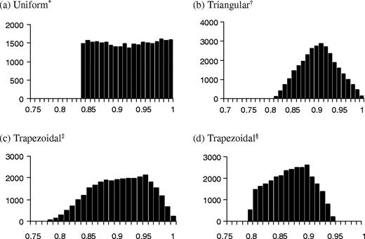
Actual output of sensitivity and specificity distributions using uniform (a), triangular (b), and trapezoidal (c and d) distributions based on 30 000 iterations. ‘*’ Sensitivity using a uniform distribution (min = 0.8, max = 1.0); ‘†’ Sensitivity using a triangular distribution (min = 0.8, mode = 0.9, max = 1.0); ‘‡’ Sensitivity using a trapezoidal distribution (min = 0.75, mode1 = 0.85, mode2 = 0.95, max = 1.0); and ‘§’ Specificity using a trapezoidal distribution (min = 0.7, mode1 = 0.8, mode2 = 0.9, max = 0.95), truncated at 0.788 to avoid negative corrected counts in the example
References
Poole C. Low P-values or narrow confidence intervals: which are more durable?
Rothman KJ, Greenland S. Approaches to statistical analysis. In: Rothman KJ, Greenland S, (eds). Modern Epidemiology. 2nd edn. Philadelphia, PA: Lippincott-Raven,
Greenland S. Basic methods for sensitivity analysis and external adjustment. In: Rothman KJ, Greenland S, (eds). Modern Epidemiology. 2nd edn. Philadelphia, PA: Lippincott-Raven,
Lash TL, Fink AK. Semi-automated sensitivity analysis to assess systematic errors in observational data.
Phillips CV. Quantifying and reporting uncertainty from systematic errors.
Greenland S. The impact of prior distributions for uncontrolled confounding and response bias: a case study of the relation of wire codes and magnetic fields to childhood leukemia.
Greenland S. Interval estimation by simulation as an alternative to and extension of confidence intervals.
Greenland S. Multiple-bias modeling for analysis of observational data (with discussion).
Thompson WD. Statistical criteria in the interpretation of epidemiologic data.
Goldberg JD. The effects of misclassification on the bias in the difference between two proportions and the relative odds in the fourfold table.
Barron BA. The effects of misclassification on the estimation of relative risk.
Gustafson P. Measurement Error and Misclassification in Statistics and Epidemiology. Boca Raton: Chapman and Hall/CRC,
Rothman KJ, Greenland S, (eds). Modern Epidemiology. 2nd ed. Philadelphia, PA: Lippincott-Raven,
Kristensen P. Bias from nondifferential but dependent misclassification of exposure and outcome.
Chavance M, Dellatolas G, Lellouch J. Correlated nondifferential misclassifications of disease and exposure: application to a cross-sectional study of the relation between handedness and immune disorders.
Dosemeci M, Wacholder S, Lubin JH. Does nondifferential misclassification of exposure always bias a true effect toward the null value?
Wacholder S, Hartge P, Lubin JH et al. Non-differential misclassification and bias towards the null: a clarification [Letter].
Jurek A, Greenland S, Maldonado G et al. Proper interpretation of nondifferential misclassification effects: expectations versus observations.
Marshall JR, Hastrup JL. Mismeasurement and the resonance of strong confounders: uncorrelated errors.
Greenland S. The effect of misclassification in the presence of covariates.
Savitz DA, Baron AE. Estimating and correcting for confounder misclassification.
Marshall JR, Hastrup JL, Ross JS. Mismeasurement and the resonance of strong confounders: correlated errors.
Jurek A, Maldonado G, Church TR et al. Exposure-measurement error is frequently ignored when interpreting epidemiologic study results [abstract].
Greenland S. Variance estimation for epidemiologic effect estimates under misclassification.
Espeland MA, Hui SL. A general approach to analyzing epidemiologic data that contain misclassification errors.
Carroll RJ, Ruppert D, Stefanski LA. Measurement Error in Nonlinear Models. Boca Raton, FL: Chapman and Hall,
Lyles RH. A note on estimating crude odds ratios in case-control studies with differentially misclassified exposure.
Cole SR, Chu H, Greenland S. Multiple-imputation for measurement error correction in pediatric chronic kidney disease [abstract].
Robins JM, Rotnitzky A, Zhao LP. Estimation of regression coefficients when some regressors are not always observed
Greenland S, Salvan A, Wegman DH et al. A case-control study of cancer mortality at a transformer-assembly facility.
Gustafson P, Greenland S. Counterintuitive phenomena in adjusting for exposure misclassification.
Lash TL, Silliman RA. A sensitivity analysis to separate bias due to confounding from bias due to predicting misclassification by a variable that does both.

