Article Text

Abstract
Objective To demonstrate an application of Bayesian model averaging (BMA) with generalised additive mixed models (GAMM) and provide a novel modelling technique to assess the association between inhalable coarse particles (PM10) and respiratory mortality in time-series studies.
Design A time-series study using regional death registry between 2009 and 2010.
Setting 8 districts in a large metropolitan area in Northern China.
Participants 9559 permanent residents of the 8 districts who died of respiratory diseases between 2009 and 2010.
Main outcome measures Per cent increase in daily respiratory mortality rate (MR) per interquartile range (IQR) increase of PM10 concentration and corresponding 95% confidence interval (CI) in single-pollutant and multipollutant (including NOx, CO) models.
Results The Bayesian model averaged GAMM (GAMM+BMA) and the optimal GAMM of PM10, multipollutants and principal components (PCs) of multipollutants showed comparable results for the effect of PM10 on daily respiratory MR, that is, one IQR increase in PM10 concentration corresponded to 1.38% vs 1.39%, 1.81% vs 1.83% and 0.87% vs 0.88% increase, respectively, in daily respiratory MR. However, GAMM+BMA gave slightly but noticeable wider CIs for the single-pollutant model (−1.09 to 4.28 vs −1.08 to 3.93) and the PCs-based model (−2.23 to 4.07 vs −2.03 vs 3.88). The CIs of the multiple-pollutant model from two methods are similar, that is, −1.12 to 4.85 versus −1.11 versus 4.83.
Conclusions The BMA method may represent a useful tool for modelling uncertainty in time-series studies when evaluating the effect of air pollution on fatal health outcomes.
- Bayesian model averaging
- Generalized additive mixed model
- PM<sub>10</sub>
- Respiratory mortality
- Time-series study
- Model uncertainty
This is an Open Access article distributed in accordance with the Creative Commons Attribution Non Commercial (CC BY-NC 4.0) license, which permits others to distribute, remix, adapt, build upon this work non-commercially, and license their derivative works on different terms, provided the original work is properly cited and the use is non-commercial. See: http://creativecommons.org/licenses/by-nc/4.0/
Statistics from Altmetric.com
- Bayesian model averaging
- Generalized additive mixed model
- PM<sub>10</sub>
- Respiratory mortality
- Time-series study
- Model uncertainty
Strengths and limitations of this study
Provide a novel modelling technique allowing for the modelling uncertainty derived from knots selection for conventional GAMM to assess the association between air pollutants and adverse health outcomes.
Provide robust effect estimation from time-series studies on PM10 and fatal health outcomes.
Uncertainty from variable selection and other sources was not investigated.
No lag effect of PM10 on respiratory mortality was examined.
Introduction
Numerous time-series studies have indicated a positive association of ambient inhalable coarse particles, including particulate matters with diameters >2.5 µm and <10 µm (PM2.5−10) and PM10 with daily respiratory death counts.1–6 In time-series studies, one major methodology concern is potential confounding due to factors that vary on similar timescales as the pollutant concentrations or outcome. Although time-series studies have substantially strengthened the evidence base for the adverse health effect of PM10, methodological development of time-series studies to better adjust for confounding is still fully justified.7 The impact of potential confounders, for example, weather and time, on the association of PM10 with mortality or other health outcomes can be non-linear and may vary with season. Thus, a wide variety of approaches have been developed and applied in modelling and estimating the non-linear functions of continuous confounders in recent years. Prominent examples are smoothing splines,8 penalised basis splines,9 adaptive regression splines10 ,11 and local polynomials.12 These methods allow for greater flexibility in data modelling, because they relax the linearity assumption traditionally required in standard parametric methods.
The generalised additive mixed model (GAMM), an extension of the generalised additive model (GAM), has become a widely used method for evaluating short-term effect of air pollution. The fact that it allows for serial correlations and spatial designs makes it a popular method in environmental epidemiological studies.13 However, often there are several competing models to select from (ie, using different combinations of confounders), and the process of selecting the best/optimal model often varies and evaluating one's ultimate selection among the others is difficult. Model uncertainty can be significant, as selection of models might lead to largely different conclusions, but often the classical approach conditioning on a single presumed model ignores or underestimates such uncertainty.14
One common way to comprehend the problem is to conduct a ‘sensitivity analysis’ using a range of different plausible models to investigate the robustness of the estimates.15 However, this still does not incorporate model uncertainty into effect estimates because it still requires selection of a single final model. To address this, researchers have proposed the Bayesian model averaging (BMA) method when assessing the triggering effect of air pollution on mortality.16 BMA is a technique designed to account for the uncertainty of the model selection process. By averaging over many different competing models, BMA incorporates model uncertainty into the estimation of parameters and prediction. BMA has been applied successfully in many statistical model classes including linear regression, generalised linear models, Cox regression models and discrete graphical models, in all cases improving predictive performance.17
Our study re-examined the association between the concentration of PM10 (including PM2.5−10) and the daily respiratory mortality rate (MR) from a time-series study design.1 The goal of this paper is to demonstrate application of BMA within the GAMM frame and provide novel modelling techniques for time-series studies. We first demonstrated the application of the BMA method in GAMM. Second, we compared the estimates of three modelling techniques, that is, generalised linear mixed model (GLMM), optimal GAMM and Bayesian model averaged GAMM (GAMM+BMA). The study was approved by the Institutional Review Board of Basic Medical Sciences, Chinese Academy of Medical Sciences, China.
Materials and methods
The data used in this study included the number of daily respiratory deaths, air quality and meteorological conditions from 1 January 2009 to 31 December 2010 in eight districts having air quality monitoring stations of a metropolitan area in Northern China. The geographic location of the eight districts was published elsewhere.1 Respiratory mortality data were obtained from the regional Causes of Death Registry (CDR). All deaths in CDR were coded according to the 10th version of the International Classification of Diseases (ICD-10). The data collection was described in detail elsewhere.1 ,18 In this study, ICD-10 codes J00–J98 were used to identify deaths due to respiratory diseases. In total, 10.38 million permanent residents and 9559 respiratory deaths were included in the study. Air quality data included the concentrations of PM10, nitrogen oxides (NOx) and carbon monoxide (CO). The daily concentrations of these pollutants were presented as an average of 24 hourly measurements. To adjust for the effect of weather conditions, data on meteorological conditions, including mean daily temperature, relative humidity, wind speed and barometric pressure during the study period, were obtained from the local meteorological administration. Previous studies conducted in the same area mostly used citywide average pollutant concentrations,19 ,20 whereas our study used pollutant concentrations measured in 11 stations of the study area and used station-specific pollutant concentrations. The spatial distribution of these monitoring stations over the districts was described elsewhere.1
The daily numbers of respiratory deaths in the eight districts were assumed to follow quasi-Poisson distribution to account for overdispersion by relaxing the distribution assumption that the variance equals the mean.21 Given the non-linear relationship of the daily number of respiratory deaths to calendar day, temperature and barometric pressure, we used GAMM to account for these non-parametric components and district-level random effect. Natural splines were used to fit the non-linear trend of the mortality, adjusting for potential confounders, that is, meteorological conditions and day of the week (DOW). The full GAMM for single-pollutant included PM10, relative humidity, wind speed, DOW, smoothing functions for calendar day, temperature and barometric pressure, as well as random effect of districts, and can be expressed as: 1where E(yi,t) is the expected number of deaths in district i on t-th day, DOW is a dummy variable for day of week, Districti is a dummy variable for the eight districts and Zi is a random intercept for districts i. s(.)s are the smoothing functions realised by natural cubic spline with n1 knots per year to adjust for long-term temporal trend, n2 knots for temperature and n3 knots for barometric pressure.22 Although natural cubic spline offers less flexibility at the limits where the second derivatives are zero, it presents a larger variance around the limits.23 We used the annual average population size of each district as the offset in the Poisson regression model.24 We also used the multipollutant model that included NOx and CO to adjust for potential confounding from other pollutants. The optimal GAMM with the most appropriate number of knots for calendar day, temperature and relative humidity was determined by minimising Akaike information criterion (AIC).25
However, because we usually have rather limited knowledge about seasonal or longer time trend in the mortality time series, knot selection in GAMM might be complicated and oversmoothing or undersmoothing the series may potentially attenuate a true pollution effect.7 In such a situation, the BMA method provides a plausible solution to incorporate the model uncertainty derived from the knot selection. The basic idea behind BMA is summarised as follows.17
Considering model Mk having the structure given by equation 1, if β is the coefficient of interest, then its posterior distribution given data D is 2
2
This is an average of the posterior distributions under each of the GAMM models considered, weighted by their posterior model probability. In equation (2), M1, …, MK are the models considered. The posterior probability for the model Mk is given by 3where Mk is one of the potential underlying models for data D with a prior probability pr(Mk) that it is true, and
 4is the integrated likelihood of model Mk. In equation (4), βk is the coefficient of model Mk, pr(βk|Mk) is the prior density of βk under model Mk, pr(D|βk, Mk) is the likelihood and all probabilities are implicitly conditional on all models being considered.
The posterior mean and variance of β are defined as: 5and
5and 6where
  .
.
The 95% Bayesian credible interval (CI) of β is 7
7
The posterior probability pr(Mk|D) in the above formula for each model was estimated by:26 8where
  is the Bayesian information criterion (BIC) of model k, which extracts a penalty according to the number of terms in the model, and
  is the average of
  (l=1,…, K).
 in equation 5 and
  in equation 6 are the posterior mean and variance of the parameter of interested, which derived from existing functions to estimate GAMMs may not correspond to the posterior mean and variance. In addition, we use BIC in equation 8 to approximate Bayes factors. Thus, the method presented here is an empirical approximation to a fully Bayesian form of model averaging, bridging classical frequentist and Bayesian estimation methods.27 ,28
In our study, the prior probability pr(Mk) was assumed to be from the uniform distribution, thus: 9
9
According to equation 5, the posteriors mean is averaged over all models, applying weights that depend on the degree to which data support each model. The weight given by equation 8 incorporates the BIC component that penalises for dimensionality of the model. Therefore, the best models are weighted heavily in equation 5 by equation 8, which in turn heavily favours parsimonious models as well.
To consider correlations between PM10 and CO and NOx, we introduced principal components (PCs) derived from principal component analysis (PCA) into the multipollutant models to exclude the impacts of collinearity between the three pollutants.18 We then transformed the regression coefficients of the PCs back to the regression coefficients of the original pollutants.
All analyses in our study were conducted in the statistical software Stata (V.14.1; StataCorp LP, College Station, Texas, USA) and using R software (V.3.2.3) packages ‘mgcv’, ‘splines’ and ‘lme4’. Since <2% of the observations in the data set were incomplete, the listwise deletion method was used to handle missing values.
Results
The daily respiratory mortality rate (per 100 000 persons) and PM10, NOx and CO concentrations of the eight districts are shown in table 1. The highest daily mortality rates were found in districts 3 (median=0.24; IQR=0.24) and 8 (median=0.25; IQR=0.25). During the 2-year study period, the annual median concentrations for PM10, NOx and CO were 106.0 μg/m3, 61.0 μg/m3 and 1.20 mg/m3, respectively. The annual median concentrations of PM10 and NOx were above the limits of Class II of the National Ambient Air Quality Standards of China (70 μg/m3 for PM10 and 50 μg/m3 for NOx), but that for CO was below the national limit (4 mg/m3).29
Daily respiratory mortality rate and PM10 concentrations by districts in the study area, 2009–2010
The meteorological conditions of the same period in the study area are shown in table 2. The mean temperature was 13.0°C ranging from −12.5°C to 34.5°C, the mean relative humidity was 51.0% ranging from 13.0% to 92.0% and the mean barometric pressure was 101.2 kPa ranging from 99.0 to 103.7 kPa, a characteristic of a typical subhumid warm continental monsoon climate.
Meteorological conditions in the study area 2009–2010
The pairwise Pearson's correlation coefficients between pollutants and meteorological conditions are shown in table 3. We observed strong linear correlation between temperature and barometric pressure (r=−0.83, p<0.001). To control for the collinearity, we included temperature, relative humidity and wind speed but not barometric pressure in the conventional GLMM analysis.
Pairwise Pearson correlation coefficients between pollutants and meteorological conditions
The observed and predicted (based on quasi-Poisson distribution) numbers of daily respiratory deaths of the eight districts between 2009 and 2010 corresponded well with no zero-inflation observed, supporting the distributional assumptions in GAMM analysis (figure 1). There were a clear temporal trend of daily number of respiratory deaths (figure 2A) and a non-linear relationship between daily number of respiratory deaths and temperature as well as barometric pressure (figure 2C, D), supporting the choice of including them as smoothing functions in GAMM. There was a moderate linear relationship of daily average relative humidity to daily number of respiratory deaths (figure 2E), and we therefore included daily average relative humidity as a linear component in the model. However, we did not observe a clear linear or non-linear relationship between daily number of respiratory deaths and wind speed (figure 2F). As a result, we included wind speed as a linear component first and as a smoothing function later in a sensitivity analysis.

Observed proportion and predicted probability based on Poisson distribution of number of daily respiratory deaths in the study area between 2009 and 2010.

Relationship between number of daily respiratory deaths and (A) days; (B) PM10 concentrations and (C–F) meteorological conditions. Lowess; locally weighted scatterplot smoothing.
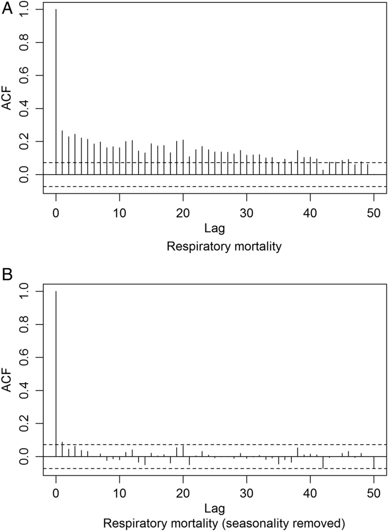
We also examined the seasonality of respiratory mortality using autocorrelation function (ACF). The slow decrease in autocorrelation from lag 1 to lag 50 shown in the correlogram (figure 3A) indicates that there is some temporal trend in the mortality series. We removed this trend by regressing the mortality against a smoothing function of time. The correlogram of the residuals after removing the seasonality (figure 3B) shows substantially less autocorrelation. Thus, season is an important factor related strongly to PM10, meteorological conditions and mortality as shown in figures 2 and 3.

ACF for respiratory mortality for (A) raw data and (B) residuals after removing seasonality. ACF, autocorrelation functions.
There were moderate to strong correlations between PM10 and CO as well as NOx (table 3), and we introduced the first and the second PCs derived from PCA into the multipollutant models. They accounted for 94.22% of variation of the three pollutants.
For GAMM analyses, we used different combinations of number of knots (from 3 or 4 to 24 knots for each smoothing function of calendar day, temperature and barometric pressure) and showed the results of combinations with the relative large posterior probability around the best model, that is, 12, 14 and 16 knots calendar day; 5, 6 and 7 knots for temperature and 4, 5 and 6 knots for barometric pressure, respectively. The knot combinations with convergence problem or extreme small posterior probability were excluded. The estimated coefficients, their corresponding SEs as well as AICs and BICs of 27 considered versions of single-pollutant (ie, PM10) GAMMs are shown in table 4. The estimated regression coefficients of PM10 changed little with different knots for barometric pressure but increased with the increasing knots for temperature. However, when the number of knots of calendar day changed from 12 to 14 and from 14 to 16, the regression coefficients of PM10 showed a slight U-shape (table 4).
Coefficients of PM10 of GAMMs for single-pollutant with different knots
Estimated increases in respiratory MR for single-pollutant, multipollutant and PCA-based multipollutant models are presented in figure 4. The same knot combination for temperature, etc, was optimal across the single-pollutant and the multipollutant models. The results of the GLMMs, optimal GAMMs and GAMM+BMA are presented of in table 5. Only GLMM of the single-pollutant model confirmed a statistically significant association between PM10 and daily number of respiratory deaths, with the largest effect of PM10 3.07 (95% CI 0.91 to 5.27) per cent increase in daily respiratory MR per IQR increase in PM10 concentration. GAMM+BMA and the optimal GAMM of single-pollutant, multipollutants and PCA-based multipollutant showed comparable results for the effect of PM10 on daily respiratory MR, that is, one IQR increase in PM10 concentration corresponded to 1.38% vs 1.39%, 1.81% vs 1.83% and 0.87% vs 0.88% increase, respectively, in daily respiratory MR (table 5). However, by incorporating the uncertainty in knots selection, GAMM+BMA gave slightly but noticeable wider CIs for the single-pollutant model (−1.09 to 4.28 vs −1.08 to 3.93) and the PCA-based model (−2.23 to 4.07 vs −2.03 vs 3.88). The CIs of the multiple-pollutant model from the two methods are similar, that is, −1.12 to 4.85 versus −1.11 versus 4.83. The results indicate that BMA provides inference about parameters taking account of the different knot selection strategies, this sometimes being an important source of uncertainty in additive model analysis, and in our example we have found that single model-based CIs tend to be narrow, which might increase the probability of false-positive finding.
Per cent increase in daily respiratory MR associated with an IQR increase in PM10 concentration from GLMM, optimal GAMM and GAMM+BMA

Estimated per cent increase in daily respiratory deaths per IQR increase in PM10 concentration in GLMM, optimal GAMM, GAMMs with different knots in day, temperature and pressure (indicated by D, T and P) and GAMM+BMA for single pollutant, multiple pollutants and PCA. BMA, Bayesian model averaging; GAMM, generalised additive mixed model; GLMM, generalised linear mixed model; PCA, principal component analysis.
In addition, the effect of the first PC in GAMM and GAMM+BMA was statistically significant (data not shown), potentially indicating a joint effect of PM10, NOx and CO on respiratory mortality. For sensitivity analysis, including wind speed as a linear component or a smoothing function in GAMM changed the results little (data not shown).
Discussion
Yang et al1 and Zhang et al30 had examined the triggering effect of PM10 on respiratory mortality in the same area previously. However, the studies were based on GAM. Although GAM is a powerful method for modelling non-linear effects of continuous covariates in regression models with non-Gaussian response, it cannot account for the between-cluster heterogeneity and within-cluster correlation of the pollutant concentrations. In recent years, smoothing based mixed model, that is, GAMM and its extensions have gained popularity in part for its ability to account for such limitations.13 ,31–33 Using a subset of multisite time-series data from Yang et al's1 study, we reinvestigated the associations between short-term exposure to ambient inhalable coarse particles PM10 and daily number of deaths from respiratory diseases. By adding the random effect of districts to the additive predictors, we used GAMM to provide a unified likelihood framework for non-parametric regression for potentially correlated exposures.13
Standard statistical methods for estimating the association between air pollutants and adverse health outcomes often fail to incorporate the model uncertainty in effect estimates. For example, knot selection for splines used in GAMM is critical, because it determines the degree of smoothness in the smoothing function of time as well as the amount of residual temporal variation in mortality. In studies using GAMM to examine effect of pollutants, we usually have rather limited knowledge about the complexity of the seasonal and long-term trends in the mortality time series or in the pollution time series. Although there are often biological or mechanistic information that is applied, current approaches in choosing the number and location of knots are mainly data-driven34 ,35 and are based on prior knowledge of the timescales where confounding is more likely to occur. More importantly, the single model selection at the end that ignores the entire process of getting to the final model and the failure to account for this uncertainty might bias our judgment.
Thus, there is concern about underestimated uncertainty in model selection in time-series air pollution studies. If a single ‘best’ model was used, the variance estimates for its coefficients will not fully reflect their true uncertainties.36 A coherent and conceptually simple way to take into account model uncertainty when making reference is BMA. In theory, BMA provides better average predictive performance than any single model, and this theoretical result has now been supported in practice in a range of applications involving different model classes and types of data.17 While BMA is an attractive solution to the problem of model uncertainty, it is not yet part of the standard data analysis tools in epidemiological studies due to several practical difficulties, including impractical exhaustive summation of posterior distribution, the computational difficulty of integrals and the challenge of specifying prior distribution over competing models. In addition, owing to lack of official solution for GAMM in common commercial statistical software, model fit criteria such as the BIC are not handily available,26 making it difficult to construct the model weight to weigh estimated coefficients of the individual models. Although Whitney and Ngo26 demonstrated the application of BMA in the GAM frame, they only examined the piece-wise linear relationship between air pollutants and mortality, essentially limiting their algorithm to a GLMM.
In our study, we demonstrated the feasibility of implementing BMA in GAMM frame in R software environment. For single-pollutant and multipollutant models, our optimal GAMM and GAMM+BMA gave equivalent point estimates for effect of PM10 on respiratory MR. Compared with previously published studies, our GAMM+BMA method for single-pollutant gave comparable results (per cent increases ranging from 0.87 to 1.38 vs 1.01 to 2.071 ,18 ,30 ,37 ,38). However, our multipollutant models showed smaller effect of PM10, which was consistent with previous findings suggesting that the effect of PM10 in multipollutant models was about two to three times smaller1 ,18 or slightly reversed.30 Although the relative increase of MR is rather small, taking into account the huge population (>10 million) in the study area, it still raises a severe public health challenge.
However, our main interest was not the estimated coefficients but the uncertainty of the estimation from different modelling strategies. The GAMM+BMA gave slightly but noticeable wider confidence even when only considering the model uncertainty from the knot. The averaged estimate across a set of potential valid models would derive more robust interval estimation for reducing the type I error. Future studies may use our technique to build a model-averaged dose–response relationship between PM10 and daily mortality to account for model uncertainty with respect to location and number of knots. Our method allows for a fully parametric characterisation of the effect of air pollutants on adverse health outcomes as well as adjusts for the non-parametric effects of other covariates.
There are also limitations in our study. First, we only considered the uncertainty from the knots selection but not from the selection of covariates and confounders, which is another major source of the uncertainty in estimating the effect of PM10. However, this limitation can be easily overcome by including different covariates and smoothing functions in the GAMM. Second, GAMM sometimes demonstrates problems in convergence and SE estimation, which might result in the failure of coefficient estimation. The data with many zeros can cause such problems in a model with a log link, because a mean of zero corresponds to an infinite range of linear predictor values. Fundamentally, it is due to lack of identifiability, and it is the case in our study. However, the problem can be addressed using stricter convergence criteria and panelised splines.39 Third, in our study, we did not investigate the lag effect of PM10 on respiratory mortality, because our interest lies on the uncertainty of the estimated association but not the association itself. However, previous studies in the same area indicated that the strongest effect of air pollutants on respiratory mortality was in day 0 (lag 0) and day 1 (lag 1), and the strongest cumulative effect was in 2-day moving average of day 0 and day 1.18 We incorporated lag 1 of PM10 concentration in the single-pollutant and multipollutant models as a sensitivity analysis and estimated effects of lag 0 PM10 on respiratory MR increase per IQR increase in lag 0 PM10 reduced to 0.79 (−1.91 to 3.55) and 1.20 (95% CI −1.93 to 4.42), respectively. Similar results were found for GAMM+BAM. Thus, the effects of PM10 need to be investigated in further GAMM+BAM with different lag structures.
In our study, we selected a uniform distribution for the prior distribution. In Bayesian statistics, the choice of the prior distribution is often controversial. Different rules for selecting priors have been suggested in the literature.40 The most intuitive solution is to use the uniform distribution as a non-informative prior when no information is available, although it does not integrate to 1 in most of the cases (this does not pose a major problem for Bayesian analyses). In view of the large sample size in our study, the data will dominate the posterior distribution (they will overwhelm the prior), so the selection of prior distribution would not pose much effect on our parameter estimation. Actually, we were informed by previous studies on the knot and variable selection, but we pretended to be uninformative in the current study in order to incorporate uncertainty (including inappropriate models) as more as possible. We would like to use informative prior distribution to narrow the range of the included models and examine performance of different prior distributions in future studies.
In conclusion, there is an increasing interest in the use of GAMM to investigate the association between short-term exposure to PM10 and adverse health outcomes in time-series studies. Epidemiology studies incorporate different modelling strategies to adjust for confounding, making it difficult to compare results across studies. Furthermore, the uncertainty of model selection has rarely been considered and quantified in these studies. Using BMA in the GAMM frame is a promising approach to investigate the association of air pollution with adverse health using time-series data, as well as other applications. Naturally, BMA tends to produce larger SE than the models that ignore model uncertainty do. However, the conclusions of BMA are more robust than those derived from analyses dependent upon a particularly selected model. Future work should aim to extend the model averaging over more extensive families of models, employing the method to explore heterogeneity in other areas (such as confounder selection), developing corresponding package in R for widespread use and exploring implications of utilising these resulting estimates of effect and corresponding uncertainty on policy-making and decision-making.
References
Footnotes
Contributors XF designed the study, did data analysis, interpreted the results and drafted the article; RL prepared the data, drafted the article and revised it critically; HK revised the article critically for important intellectual content; MB provided statistical consultation and revised the article critically; FF and YC are the guarantors of the study, and they monitored the study implementation and revised the article critically for important intellectual content. All authors contributed to further drafts and approved the version to be published.
Funding The authors gratefully acknowledge research grants to YC from the Junior Faculty Research Grants (C62412022) of the Institute of Environmental Medicine, Karolinska Institutet, and from the fund for PhD research (KID-funds) and travel (KI-foundations and funds) of Karolinska Institutet, Sweden, and research grants to RL from the Public Welfare Research Program of National Health and Family Planning Commission of China (201402022) and from the Opening Project of Shanghai Key Laboratory of Atmospheric Particle Pollution and Prevention (LAP3).
Disclaimer The funding sponsors had no role in the design of the study, in the collection, analysis or interpretation of data, in the writing of the manuscript or in the decision to publish the research results.
Competing interests None declared.
Ethics approval Institutional Review Board of Basic Medical Sciences, Chinese Academy of Medical Science, China.
Provenance and peer review Not commissioned; externally peer reviewed.
Data sharing statement No additional data are available.