Article Text

Abstract
Objective Body mass index (BMI) may cluster in space among adults and be spatially dependent. Whether and how BMI clusters evolve over time in a population is currently unknown. We aimed to determine the spatial dependence of BMI and its 5-year evolution in a Swiss general adult urban population, taking into account the neighbourhood-level and individual-level characteristics.
Design Cohort study.
Setting Swiss general urban population.
Participants 6481 georeferenced individuals from the CoLaus cohort at baseline (age range 35–74 years, period=2003–2006) and 4460 at follow-up (period=2009–2012).
Outcome measures Body weight and height were measured by trained healthcare professionals with participants standing without shoes in light indoor clothing. BMI was calculated as weight (kg) divided by height squared (m2). Participants were geocoded using their postal address (geographic coordinates of the place of residence). Getis-Ord Gi statistic was used to measure the spatial dependence of BMI values at baseline and its evolution at follow-up.
Results BMI was not randomly distributed across the city. At baseline and at follow-up, significant clusters of high versus low BMIs were identified and remained stable during the two periods. These clusters were meaningfully attenuated after adjustment for neighbourhood-level income but not individual-level characteristics. Similar results were observed among participants who showed a significant weight gain.
Conclusions To the best of our knowledge, this is the first study to report longitudinal changes in BMI clusters in adults from a general population. Spatial clusters of high BMI persisted over a 5-year period and were mainly influenced by neighbourhood-level income.
- EPIDEMIOLOGY
- PUBLIC HEALTH
- NUTRITION & DIETETICS
This is an Open Access article distributed in accordance with the Creative Commons Attribution Non Commercial (CC BY-NC 4.0) license, which permits others to distribute, remix, adapt, build upon this work non-commercially, and license their derivative works on different terms, provided the original work is properly cited and the use is non-commercial. See: http://creativecommons.org/licenses/by-nc/4.0/
Statistics from Altmetric.com
Strengths and limitations of this study
As far as we know, this is the first study to report the persistence of spatial clusters of high body mass index (BMI) values over a 5-year period in adults from a general population.
The observed east-to-west pattern of BMI clustering fits known socioeconomic and ethnocultural differences distinguishing these opposite regions of the city of Lausanne, Switzerland.
A consequence of the social policy applied by the city is likely to fix populations with modest income in subsidised housing located in specific areas.
While recruitment methods of the CoLaus study aimed at collecting information on a representative sample of the general population, adult participants and non-participants to the CoLaus study may differ, and participation bias cannot be excluded.
We considered several individual-level covariates, but data on individual income was missing. We used, instead, the median income of the including city statistical sector.
Introduction
Elevated body mass index (BMI) is a major risk factor for cardiovascular diseases, diabetes, cancers and all-cause mortality.1 Growing evidence shows that adults with a high BMI tend to cluster in space among adults, and that the distribution of BMI is spatially dependent.2 ,3 To explore the link between the place of residence and health, spatial analysis methods have been developed and introduced in epidemiological research.4 Spatial clusters of a trait can be determined by its spatial dependence (spatial autocorrelation), defined as a covariation of properties, such as BMI, within a geographic space. Previous reports have used spatial analyses to identify clusters of obesity and obesity-related factors among adult populations.2 ,5 ,6 Using a large adult population-based study in the State of Geneva, Switzerland, Guessous et al3 showed that BMI levels were not randomly distributed across the State, but that in specific areas an individual's BMI was associated with the mean BMI of the neighbourhood. Significant clusters of high and low BMIs were identified. Further, BMI levels appeared to be spatially dependent according to community characteristics.7 Although a number of neighbourhood-related risk factors of obesity exist, income level is thought to be of major importance3 while associations between other community environmental attributes and obesity have been inconsistent. Yet, the potential impact of income on the spatial dependence of BMI levels has been rarely assessed. For instance, a reduction of BMI clustering after adjustment for the area-level income would suggest that neighbourhood socioeconomic characteristics may impact individual's BMI directly, especially if this attenuation is independent of individual-level factors such as age, physical activity and individual socioeconomic status.3
So far, studies specifically exploring the spatial distribution of BMI clusters in adults have been limited by their cross-sectional design.8–10 Similarly to what is being done for infectious diseases, considering the spatial dynamics of BMI clusters using longitudinal data could further improve our understanding of the association of urban environment and neighbourhood socioeconomic context with obesity. This could also be an effective approach to develop interventions that better take the space and temporal variations into consideration.
In this study, we determine the 5-year changes in spatial dependence of BMI, and the BMI spatial dependence among participants who developed obesity, applying a spatial analytic approach to a Swiss urban population-based cohort with longitudinal data on measured BMI at the individual level. Further, we assessed the extent to which BMI special dependence is accounted for by socioeconomic factors at the neighbourhood and individual levels.
Methods
CoLaus
We used the data from the CoLaus baseline and follow-up study. The primary aims of the CoLaus study were to assess the prevalence and determinants of cardiovascular disease in the Caucasian population of Lausanne, Switzerland.11 The CoLaus study complied with the Declaration of Helsinki and was approved by the local Institutional Ethics Committee. All participants gave written informed consent. The sampling procedure of the CoLaus study has been described elsewhere.11 Briefly, the CoLaus study was population-based and included participants aged 35–75 years at baseline (2003–2006). The recruitment took place in the city of Lausanne in Switzerland, a town of 126 700 inhabitants (as of December 2003). The complete list of the Lausanne inhabitants aged 35–75 years was provided by the population register of the city. A simple, non-stratified random sample of 35% of the overall population was drawn. The sample of 8121 individuals who agreed to participate represented 41% of the initially sampled population. The baseline CoLaus study enrolled 6733 participants (3544 women) of whom 5064 participants were willing to be recontacted for the follow-up (2009–2012). At baseline and follow-up, participants attended a single visit at the Centre Hospitalier Universitaire Vaudois, which included an interview and a physical examination. Average follow-up time was 5.5 years.
Body weight and height were measured by trained healthcare professionals with participants standing without shoes in light indoor clothing. BMI was calculated as weight (kg) divided by height squared (m2). Self-reported information on education level (5 categories based on the highest level of education achieved), ethnicity (Caucasian vs non-Caucasian), marital status (living alone vs living in couple), receiving government benefits (yes, no), physical activity (4 categories based on the response to the following question: ‘How many times per week do you take part for at least 20 min in leisure-time physical activity?’), smoking status (current, former, non-smoker) and alcohol consumption (yes, no).
Geocoding
Geocoding was performed using QGIS (Quantum GIS Development Team, 2013) with the extension MMQGIS (http://michaelminn.com/linux/mmqgis/) containing a geocoding Python plugin facilitating the use of the Google Maps API. We took into consideration for analysis individuals sampled in the urban area only (further details in online supplementary material).
Neighbourhood-level income
To assess the impact of an area's income level on BMI spatial dependence, we compared results with and without BMI adjustment for the area's income. Data on area's income level were obtained from the 2009 Lausanne Census (Office Cantonal de la Statistique, http://www.scris-lausanne.vd.ch). Information on median annual income in Swiss francs CHF (1 CHF= US$1.02, September 2015) covered 81 statistical sectors of the city (average population of the statistical sectors is 1687). The income value was attributed to individuals on the basis of the inclusion of their postal address (place of residence) within the corresponding sector. Online supplementary figure S1 shows a box map of the median income in 2009 per statistical sector (81) in the city of Lausanne.
Individual socioeconomic and demographic status
To assess the potential impact of individual-level characteristics (including socioeconomic status) on BMI spatial dependence, we ran additional models further adjusted for age, sex, education level, Caucasian ethnicity, marital status, government benefits, physical activity, smoking status and alcohol consumption.
Spatial dependence of BMI among participants with weight gain
We then explored the spatial dependence of follow-up BMI among participants showing a BMI increase ≥5% between baseline and follow-up as used elsewhere.12 Models with raw BMI, BMI adjusted for neighbourhood-level median income, and BMI further adjusted for individual-level characteristics were used.
Spatial analysis
Using the geographical coordinates of the postal addresses (place of residence), we applied the Getis-Ord Gi statistic13 ,14 implemented in the GeoDa software15 to detect where in the city clustering of high BMI values may be occurring. Getis-Ord Gi indicators are statistics that measure spatial dependence and evaluate the existence of local clusters in the spatial arrangement of a given variable (here BMI). They compare the sum of an individual's BMI values included within a given spatial lag proportionally to the sum of the individual's BMI values within the whole study area.13 Further details are available in the online supplementary material. The Gi statistic is a Z score. The null hypothesis for this statistic is that the values being analysed exhibit a random spatial pattern. Statistical significance testing was here based on a conditional randomisation procedure16 using a sample of 999 permutations, and based on the Bonferroni/Sidak procedure to correct for multiple comparisons.16 All maps shown in this paper correspond to a significance level of 0.05 (see figure 5 in ref. 17), with online supplementary figure S2 illustrating how much the significance may vary according to different α levels. Large statistically significant positive and, respectively, negative Z scores reveal clustering of high and, respectively, low BMI values. A hot spot13 is a statistically significant cluster of high values. A cold spot is a statistically significant cluster of low values. All sampling sites which are not significant are displayed in white. We analysed the BMI variables within 800 m around each individual's residence (ie, spatial lag). Quantile regression was used to generate residuals to obtain adjusted BMI.18
To test the robustness of our findings, we ran the following additional sensitivity analyses: (1) analyses of baseline BMI cluster restricted to participants who also attended the follow-up examination, (2) all analyses restricted to participants living in the urban area of the city and who did not change residence between baseline and follow-up (N=3950), (3) analyses implementing BMI adjustment with different covariates (eg, education level and median income; education level only; all socioeconomic variables, etc) and (4) we tested eight other spatial lags (400, 600, 1000, 1200, 1400, 1600, 1800 and 2000 m). Finally, as Moran's I method, unlike Getis-Ord Gi, also identifies dissimilar values among the local high and low spots (high–low and low–high), and thus preventing misclassification of individuals in areas with relatively high numbers of dissimilar neighbouring individuals, we also ran local Moran's statistics (detailed in online supplementary material). Results provided similar patterns (see online supplementary figures S3a, b, S4a, b and S5a, b).
Results
Among the 6733 participants at baseline, 252 (3.7%) were excluded because they lived in municipal districts in the countryside, and 17 (0.25%) could not be geocoded. Thus, 6481 (96%) participants living in the urban area of Lausanne were geocoded using their postal address (geographic coordinates of the residence).
Among the 5064 participants at follow-up, 604 (12%) were excluded because they had moved outside the urban limits of the Lausanne municipality between 2006 and 2009. Thus, 4460 (88%) participants could be geocoded at follow-up.
The 17 urban districts (‘quartiers’ shown in figures 1⇓–3) contain between 2 and 10 statistical sectors (shown in online supplementary figure S1). The statistical sectors contain between 0 (for seven of them) and 328 individuals at baseline (mean=77.1; median=70) and between 0 (for eight of them) and 222 individuals at follow-up (mean=55.06; median=49). Baseline individual characteristics of participants included at baseline and at follow-up were similar (see online supplementary table S1).

Clusters for baseline showing the raw body mass index (BMI) (A) and the BMI adjusted for median income (B). White dots show sampling places where the space is neutral (no spatial dependence). Red dots show individuals with a statistically significant positive Z score (α=0.05), meaning that high values cluster within a spatial lag of 800 m, and are found closer together than expected if the underlying spatial process was random. Blue dots show individuals with a statistically significant negative Z score (α=−0.05), meaning that low values cluster within a spatial lag of 800 m, and are found closer together than expected if the underlying spatial process was random. Lausanne districts are numbered from 1 to 17. For an exact description of the limits of the districts see online supplementary figure S1. The background of the map was built on the basis of LIDAR data (height's model, Source: Géodonnées Etat de Vaud, 2012).
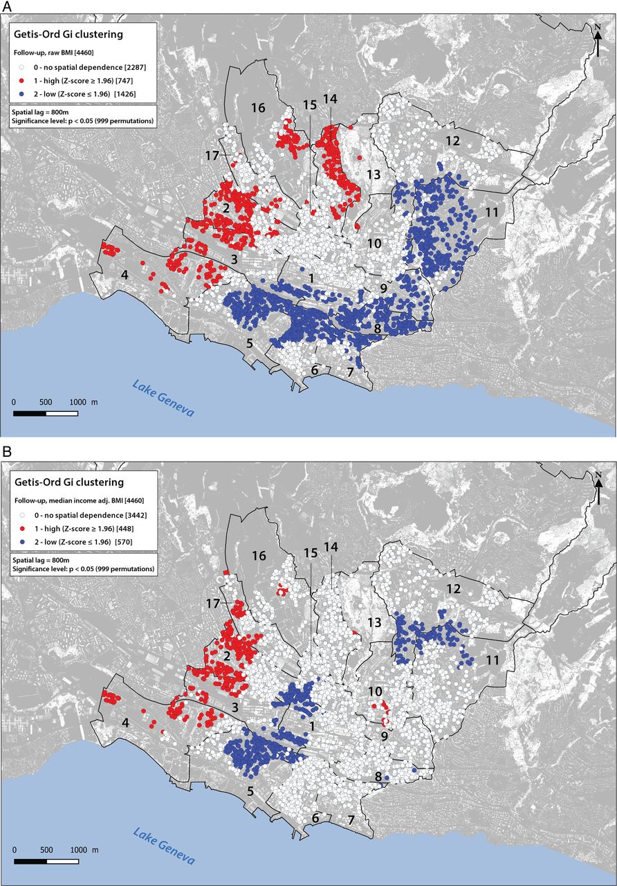
Clusters for follow-up showing the raw body mass index (BMI) (A) and the BMI adjusted for median income (B). White dots show sampling places where the space is neutral (no spatial dependence). Red dots show individuals with a statistically significant positive Z score (α=0.05), meaning that high values cluster within a spatial lag of 800 m, and are found closer together than expected if the underlying spatial process was random. Blue dots show individuals with a statistically significant negative Z score (α=−0.05), meaning that low values cluster within a spatial lag of 800 m, and are found closer together than expected if the underlying spatial process was random. Lausanne districts are numbered from 1 to 17. For an exact description of the limits of the districts see online supplementary figure S1. The background of the map was built on the basis of LIDAR data (height's model, Source: Géodonnées Etat de Vaud, 2012).

Clusters for follow-up showing the raw body mass index (BMI) (A) and the BMI adjusted for median income (B) among participants showing weight gain (≥5% of BMI increase between baseline and follow-up). White dots show sampling places where the space is neutral (no spatial dependence). Red dots show individuals with a statistically significant positive Z score (α=0.05), meaning that high values cluster within a spatial lag of 800 m, and are found closer together than expected if the underlying spatial process was random. Blue dots show individuals with a statistically significant negative Z score (α=−0.05), meaning that low values cluster within a spatial lag of 800 m, and are found closer together than expected if the underlying spatial process was random. Lausanne districts are numbered from 1 to 17. For an exact description of the limits of the districts see online supplementary figure S1. The background of the map was built on the basis of LIDAR data (height's model, Source: Géodonnées Etat de Vaud, 2012).
The mean (±SD) age of the 6481 (52.7% women) and 4460 (54.1% women) participants included at baseline and at follow-up was 52.6±10.7 and 58.1±10.5 years, respectively. The mean (±SD) BMI was 25.8±4.5 (median=25.2) and 26.2±4.6 (median=25.6) kg/m2 at baseline and follow-up, respectively, and the prevalence of obesity was 15.4% and 17.4% at baseline and at follow-up, respectively. Median (minimum–maximum range) area's annual income level was 50 882 CHF (31 306–98 586 CHF) at baseline, and 51 139 CHF (31 306–98 586 CHF) at follow-up.
Spatial dependence of BMI at baseline
Gi clusters for the 6481 adults at baseline are shown in figure 1A, B. With regard to raw BMI, 2935 (45.2%) individuals presented no BMI spatial dependence, 1224 (18.9%) belonged to spatial clusters where individuals locally showed a BMI proportionally higher than within the whole study area (high BMI cluster class or hot spots); 2322 (35.8%) belonged to spatial clusters where individuals locally showed a BMI proportionally lower than within the whole study area (low BMI cluster class or cold spots). Clear BMI clusters were identified, with hot spots predominantly in the northwest and in western districts (2–4 and 14), and cold spots predominantly in the eastern districts (5–9, 11 and south of 12) of the city.
The impact of neighbourhood-level income on spatial dependence of BMI is shown on figure 1B. Adjustment for neighbourhood-level income globally attenuated the high BMI cluster areas (14.9% instead of 18.9% of individuals). Attenuation was important in the north (district 14), but did not affect the same category of cluster in the west (districts 2–4). The adjustment attenuated low BMI cluster areas (18.4% instead of 35.8% of individuals), in particular in the east (districts 7–9 and 11), while one emerged in the centre of the city (district 1). Further adjustment for individual-level characteristics (age, sex, education level, Caucasian ethnicity, marital status, government benefits, physical activity, smoking status and alcohol consumption) only slightly changed BMI spatial dependence (see online supplementary figure S6).
In unadjusted analyses the global Moran's I (see online supplementary material) was 0.011, and 0.0044 after adjusting for neighbourhood-level median income, which is close to spatial independence in both cases. These significant values of Moran's I (p=0.01) show a decrease of global spatial autocorrelation between the two situations but above all highlight the local regime of spatial dependence in the distribution of BMI values.
Spatial dependence of BMI at follow-up
BMI spatial dependence, BMI cluster areas and the impact of neighbourhood-level income at follow-up, were very similar to those at baseline, albeit less pronounced (figure 2). With regard to raw BMI (figure 2A), 2287/4460 (51.3%) individuals presented no BMI spatial dependence; 747 (16.7%) were in the high BMI cluster class; 1426 (32.0%) were in the low cluster class. High BMI clusters were predominantly located in the northwestern districts (2–4, 14 and 16), while the low BMI clusters were predominantly located in the southeastern districts (5–9 and 11) of the city. The adjustment for neighbourhood-level income globally attenuated the high BMI cluster areas (10% instead of 16.7% of individuals). These hot spots persisted in the west (districts 2–4, 17), the high cluster in the north disappeared (14), while part of the cold spots in the east were attenuated, especially in districts 6–9 and 11 (for a global decrease from 32% to 12.7%, see figure 2B). Further adjustment for individual-level characteristics (age, sex, education level, Caucasian ethnicity, marital status, government benefits, physical activity, smoking status and alcohol consumption) did not meaningfully change BMI spatial dependence (see online supplementary figure S7).
At follow-up, the global Moran's I was 0.0094, and 0.0031 after adjusting for neighbourhood-level median income. These values show a decrease of global spatial autocorrelation in the adjusted case, but here again highlighting a behaviour close to spatial independence in the two situations.
Spatial dependence of BMI among participants showing weight gain
Weight gain (≥5% of BMI increase between baseline and follow-up) was found in 1351 adults (maximum BMI increase=35.6%, mean=9.73, median=8.24; 59% women, mean age 50.76±10.1), and was spatially scattered all over the city. Among these adults, 1109 (82.1%) individuals presented no spatial dependence in raw BMI, 107 (7.9%) belonged to spatial clusters where individuals locally showed a BMI increase proportionally higher than within the whole study area (hot spot), and 135 (10%) belonged to spatial clusters where individuals locally showed a BMI increase proportionally lower than within the whole study area (cold spot) (figure 3A). Hot spots were distributed in the west (districts 2–4, and 16) and in the centre to a lesser extent (districts 1 and 10), whereas cold spots were distributed mainly in the east (districts 8, 9 and 11), with a central spot too (districts 1, 3 and 5). Adjustment for neighbourhood-level income (figure 3B) did not change the general spatial pattern described above, but altered the intensity of spatial dependence. Indeed, 105 (instead of 107) individuals constituted stable hot spots in the west, while 162 (instead of 135) formed cold spots. The latter are concentrated in the central part of districts 1, 2, 3 and 15. In the eastern part of the city (districts 8, 9 and 11), median income cancelled 72% (61/84) of the cold spots. Finally, adjusting for individual-level characteristics (see online supplementary figure S8) globally neutralised the local BMI clusters aforementioned but led to the emergence of a cold spot in the north (57 individuals).
Sensitivity analyses restricted to participants living in the urban area of the city and who did not change residence between baseline and follow-up (N=3950) and analyses using different adjustment models provided similar results (maps available on request).
Discussion
Using repeated georeferenced measurements of BMI at the individual level in adults from the general population, we identified clusters highlighting a particular structure in the spatial distribution of high and low BMI values in the city of Lausanne. In adults, BMI is not distributed at random and shows a spatial dependence. Using longitudinal data, we also found that clusters of low and high BMI did not change in a 5-year period. Also, neighbourhood-level income clearly influenced BMI spatial dependence independently of individual-level characteristics.
In line with previous cross-sectional studies, we found spatial clustering of BMI in adults from the general population.2 ,3 ,5 ,6 ,8 Our results extend these previous findings by identifying clear high and low BMI clusters in a city of Switzerland that is characterised by a low prevalence of obesity compared to international estimates,19 a low level of social inequality (as measured by the Gini coefficient), one of the longest life expectancy in the world,20 and a universal health insurance coverage. We observed an east-to-west pattern of BMI clustering. Indeed, socioeconomic and ethnocultural differences between the east and west of the city of Lausanne are known (see http://www.scris-lausanne.vd.ch/). In the west live a majority of migrant workers, usually of Mediterranean origin. In the east live mostly Swiss citizens and people with a higher level of education. Workers and subordinates are more numerous in the west than in the east where business leaders and executives are more numerous.
Generally, association studies on BMI did not account for spatial information and assumed independence across observations. Our results are in line with a recent report,3 and clearly show that this assumption is not correct. This may explain some of the inconsistencies reported on the impact of social and built environment on obesity.21
The previously mentioned cross-sectional studies and other studies on BMI clustering conducted in various populations6 ,10 ,22–24 used self-reported BMI. Similarly to Drewnowski et al,25 we used measured BMI allowing us to estimate unbiased BMI. In addition, while previous studies have analysed single time points, we reported spatiotemporal information. At baseline and after a 5-year period, significant clusters of high versus low BMIs were clearly identified and persisted between the first and the second periods. To the best of our knowledge, this is the first study to report longitudinal BMI spatial clustering in the general adult population. An increasing body of evidence shows that neighbourhood socioeconomic context, measured by neighbourhood deprivation, neighbourhood segregation, or population density predicts the development of obesity and other related health outcomes.26 ,27 Poorer physical infrastructures and transports, worse housing conditions, fewer health and community services, and lower stocks of social capital in poor neighbourhoods are factors that have been proposed to explain how the place of residence might directly affect health.28 In addition, network phenomena, including social network, appear to be crucial factors in the biological and behavioural traits of obesity as it seems to spread through social ties.29 While all these factors are potentially dynamic, our study showed that BMI clusters remained static within the 5-year interval, suggesting a stable distribution of individual-level and neighbourhood-level characteristics in the city of Lausanne within this time frame.
Our longitudinal data also enabled the mapping of weight gain (≥5% of BMI increase), which appeared to be spatially scattered all over the city. In addition, we found that even among participants who gained weight, clusters of high and low BMI could be identified, and that these clusters corresponded—albeit less pronounced—to BMI clustering found among all participants. This is the first study to explore and report such correspondence of BMI clustering. This result suggests that the spatial clustering of high and low BMI observed in the general adult population remains identical among the limited group of persons having gained weight between baseline and follow-up: individuals gained more weight where high BMI clusters were observed among all participants.
It is well acknowledged that both individual-level and neighbourhood-level attributes can contribute to the spatial clustering of BMI.9 We used neighbourhood median income to characterise neighbourhood environment. Neighbourhood-level income is often used to identify variations in health behaviours and outcomes.30 Neighbourhood-level income was recently identified as an effect modifier of the relationships of food environments with BMI z-score among children.31 Although many other attributes such as the built environmental features have been used to characterise neighbourhood, associations between such environmental attributes and obesity have been inconsistent.22 ,23 ,32 ,33 Interestingly, residential property values were related to high and low BMI clusters in a recent study of 1602 adults included in the 2008–2009 Seattle Obesity Study, whereas built environment features were not.24 In our study, we lack information on residential property value—known to be a strong independent predictor of BMI34—but it is very likely that neighbourhood median income is highly correlated with residential property value, which could explain—at least in part—the major effect of neighbourhood median income on BMI spatial dependence observed in our study. Indeed, the city of Lausanne is an important land owner, and a consequence of the social policy applied may fix populations with modest income in subsidised housing located in the specific areas where the clusters of high BMI values were detected. Of note, we showed that further adjustment for individual-level characteristics had a minor influence on BMI spatial dependence. In fact, adjustment for individual-level characteristics had also a minor influence on raw BMI spatial dependence (maps not shown, available on request). This can be related to findings from Huang et al24 showing that high and low obesity clusters were only attenuated after adjusting for individual-level characteristics and disappeared once neighbourhood residential property values and residential density were included in the model. On the other hand, our results and Huang et al report contrast with results from a cross-sectional analysis using Northern California, USA, Kaiser Permanente data from 15 854 adults with diabetes showing that adjusting for neighbourhood-level factors reduced BMI clustering by 50%, whereas adjusting for individual-level characteristics reduced BMI clustering by 68%.9 To better disentangle the role of individual-level and neighbourhood-level characteristics on BMI spatial dependence, further spatial studies with both neighbourhood-level and individual-level indicators should be conducted, particularly if also including individual-level income which was not available in this study. While doing so, other factors (eg, built areas vs green spaces, services, transportations) that could explain, at least in part, the observed spatial dependence should be considered. For example, Hollands et al35 conducted a spatial analysis of the association between restaurant density and BMI in Canadian adults, and found that fast-food restaurant density was positively associated with BMI, independently of individual-level characteristics.
Our spatial approach allowed us to detect different patterns within statistical sectors that may have not been identified based on aggregated data. Georeferenced data enabling the characterisation of health risk factors or disease is increasingly used, and has been proposed as a tool to guide public health interventions.36 The use of such information to contextualise BMI values like in the present study can have potential impacts. It could lead to specific recommendations for future healthy urban planning (type of housing, food environment and type of urban environment37). In particular, high BMI clusters that persisted after adjustment for individual-level and neighbourhood income deserve to be further considered as they might be related to other obesogenic factors such as the food environment. The use of spatial approaches can allow identifying specific areas where to intervene and to support specific prevention campaigns, for example. Such models are being used in the UK to identify areas where antiobesity policies should be implemented.29 In addition to improving interventions, the dynamic surveillance of BMI clusters can also contribute to determining the effectiveness of such interventions.
Study limitations
We chose to use an 800 m spatial lag, but other choices may produce slightly different results. Yet, we tested the robustness of our findings using different spatial lags and found no meaningful difference in the results (clusters). We preferred the Getis-Ord Gi statistic to other statistics such as Moran's I as our interest focused primarily on the detection of local clusters of high and low BMI values.
While recruitment methods of the CoLaus study aimed at collecting information on a representative sample of the general population, adult participants and non-participants to the CoLaus study may differ and participation bias cannot be excluded (for instance, individuals residing in the same household could have participated in the study). We considered several individual-level covariates, but other data such as individual income were not available, and population density not accounted for; thus, residual confounding cannot be excluded. While reports suggest that neighbourhood-level and individual-level income are comparable in terms of ability to identify variations in outcomes,38 individual-level income should ideally be considered as neighbourhood-level and individual-level income might measure different constructs.
Conclusion
To the best of our knowledge, this is the first study to explore longitudinal changes in the spatial distribution of BMI geocoded at the postal address level (geographic coordinates of the residence). While previous studies have analysed single time points, the spatiotemporal approach proposed here identified persistent clusters with high BMI. These results suggest that specific prevention interventions involving urban planning decisions could be targeted to such areas. Further studies are needed to better understand the causes of such clustering, both at the individual level and at the structural level, and to plan interventions aiming at modifying these determinants.
Acknowledgments
The authors are grateful to the participants of the CoLaus study and to the investigators, in particular Prof Martin Preisig.
References
Supplementary materials
Supplementary Data
This web only file has been produced by the BMJ Publishing Group from an electronic file supplied by the author(s) and has not been edited for content.
- Data supplement 1 - Online supplement
Footnotes
Contributors SJ, SD and IG designed the research; SJ, SD and IG analysed the data and wrote part of the paper; SJ and IG wrote the paper. SJ, IG, PM-V, GW and PV collected the data. SJ, SD, IG and J-MT were responsible for the preparation of data. All the authors undertook revisions, contributed intellectually to the development of this paper and approved the final manuscript. IG is the guarantor.
Funding The CoLaus study was supported by research grants from GlaxoSmithKline, the Faculty of Biology and Medicine of Lausanne, Switzerland, and the Swiss National Science Foundation (grants 33CSCO-122661, 33CS30-139468 and 33CS30-148401). SS is supported by an Ambizione Grant (n PZ00P3_147998) from the Swiss National Science Foundation.
Competing interests GW reports unrestricted grant from GlaxoSmithKline, and grants from Swiss national Science Foundation, during the conduct of the study.
Ethics approval The CoLaus study complied with the Declaration of Helsinki and was approved by the local Institutional Ethics Committee.
Provenance and peer review Not commissioned; externally peer reviewed.
Data sharing statement No additional data are available.