Article Text

Abstract
Introduction and motivation Many health studies measure a continuous outcome and compare means between groups. Since means for biological data are often difficult to interpret clinically, it is common to dichotomise using a cut-point and present the ‘percentage abnormal’ alongside or in place of means. Examples include birthweight where ‘abnormal’ is defined as <2500 g (low birthweight), systolic blood pressure with abnormal defined as >140 mm Hg (high blood pressure) and lung function with varying definitions of the ‘limit of normal’. In vulnerable populations with low means, for example, birthweight in a population of preterm babies, a given difference in means between two groups will represent a larger difference in the percentage with low birthweight than in a general population of babies where most will be full term. Thus, in general, the difference in percentage of patients with abnormal values for a given difference in means varies according to the reference population’s mean value. This phenomenon leads to challenges in interpreting differences in means in vulnerable populations and in defining an outcome-specific minimal clinically important difference (MCID) in means since the proportion abnormal, which is useful in interpreting means, is not constant—it varies with the population mean. This has relevance for study power calculations and data analyses in vulnerable populations where a small observed difference in means may be difficult to interpret clinically and may be disregarded, even if associated with a relatively large difference in percentage abnormal which is clinically relevant.
Methods To address these issues, we suggest both difference in means and difference in percentage (proportion) abnormal are considered when choosing the MCID, and that both means and percentages abnormal are reported when analysing the data.
Conclusions We describe a distributional approach to analyse proportions classified as abnormal that avoids the usual loss of precision and power associated with dichotomisation.
- statistics & research methods
- epidemiology
- public health
This is an open access article distributed in accordance with the Creative Commons Attribution Non Commercial (CC BY-NC 4.0) license, which permits others to distribute, remix, adapt, build upon this work non-commercially, and license their derivative works on different terms, provided the original work is properly cited, appropriate credit is given, any changes made indicated, and the use is non-commercial. See: http://creativecommons.org/licenses/by-nc/4.0/.
Statistics from Altmetric.com
Strengths and limitations of this study
Addresses a challenging issue in study design and analysis.
Motivated by real study data and illustrated using hypothetical data to allow generalisation.
Describes a statistically robust methodological solution.
A formal review of dichotomisation was not included.
Facilitates the reporting of clinically meaningful results.
Introduction
When we design a new research study, such as a clinical trial, we usually calculate the sample size required to answer the key research questions with adequate precision and/or statistical power. When two groups are being compared, we normally consider what is the minimum difference between the groups that is clinically important. This minimum difference, sometimes referred to as the ‘minimal clinically important difference’ (MCID)1, is usually identified using clinical experience together with data from patient studies. Recommended MCIDs have been published for different outcomes in different settings such as pain scores,2 health-related quality of life,3 chronic obstructive pulmonary disease (COPD) outcomes,4 6 min walk distance5 and more. In this paper, we discuss the challenges in interpreting MCIDs which have been designed for a general population when they are applied to a vulnerable population.
Clinically meaningful effect size
Cohen suggested the use of a standardised effect size, calculated as the difference in means divided by the SD at baseline.6 He attached descriptors to different sizes of these quantities such that an effect size of 0.8 is ‘large’, 0.5 is ‘medium’ and 0.2 is ‘small’. These descriptors implicitly assume that MCID is the same for all populations, but this is not necessarily so, as we later illustrate.
When a study’s primary outcome is continuous and the clinically meaningful difference is uncertain, statisticians and researchers may express the difference to be detected as a multiple of the SD, as described above after Cohen. Hence studies sometimes set out to be able to detect, for example, a difference of 0.33 or 0.5 SD. This seems reasonable if there are no other data to inform the decisions, but behind this seemingly objective measure, the question arises of what is the meaning of a small difference? More importantly, we consider whether the clinical impact of a given difference is the same in different populations. A simple example is to consider the effect of maternal smoking in pregnancy which is associated with reduced mean birthweight of around 180 g.7 However, it is not straightforward to interpret this difference because in full-term pregnancies with mean birthweight of 3400 g, a mean reduction of 180g to 3220 g has much less clinical impact on overall pregnancy outcome than if the population were preterm babies with a mean of 2600 g reduced to 2420 g. If we think at the population level and consider a difference in means as a shift in mean,8 then translating this shift into the risk for an individual is not intuitive unless we define the percentages who are ‘abnormal’ using a clinically meaningful cut-point, such as here using birthweight <2500 g to define ‘abnormal’.
Motivating example: lung function z-scores
The phenomenon described above came to our attention while analysing and interpreting lung function z-score outcomes in children who had been born very prematurely and so from hereon we will use lung function z-scores to illustrate the problem introduced above. Z-scores are commonly used for standardising lung function measurements for age/sex/height and sometimes ethnicity. By standardising, a patient’s individual lung function measurement can be compared against a known expected value, usually in a general population. Z-scores are used in assessing an individual patient’s measurements to allow clinicians to identify abnormal values that might indicate the need for further intervention. However, in addition to their clinical use on an individual basis, z-scores are also used in research studies to compare groups, so that key demographic characteristics do not confound group-level comparisons. The simplest version of an individual’s z-score is:

where the expected value (ie, the population mean value) and SD refer to a general population with similar characteristics to the observed individual. Z-scores may be calculated using simple or complex regression modelling, for example, in standardising a child’s lung function measurement for their age, sex, height and ethnicity.9 In a sample of healthy patients, we expect their mean z-score to be close to the population mean of all individuals and so the sample mean z-score is expected to be 0 with SD equal to 1.
Hypothetical example: interpreting differences in z-scores
We conducted a brief descriptive review of the use of z-scores to see how researchers analysed and reported lung function z-scores. This indicated that where authors discussed the magnitude of group differences in mean z-scores, they tended to provide an estimate of the percentage with abnormal measurements using a clinically meaningful cut-point. Abnormal lung function z-score may be defined using one of the lower centiles of a general (normal) population, such as below 2.5th (z< -1.96) or below fifth centiles (z< -1.64).9 To illustrate these ideas, we will use the fifth centile in a general population (z< -1.64) so the cut-point is −1.64, meaning that someone with a lung function z-score less than −1.64 will be categorised as ‘abnormal’, sometimes known as ‘below the limit of normal’.
In figures 1–3, we consider three hypothetical z-score populations. Each is assumed to follow a Normal distribution with the same SD but with different means: Figure 1 mean=0 (‘general population’), figure 2 mean=−0.5 (‘moderately vulnerable population’), figure 3 mean=−1.0 (‘vulnerable population’). We see that the percentage of the population that is classed ‘abnormal’ (z< -1.64) varies with the population mean.
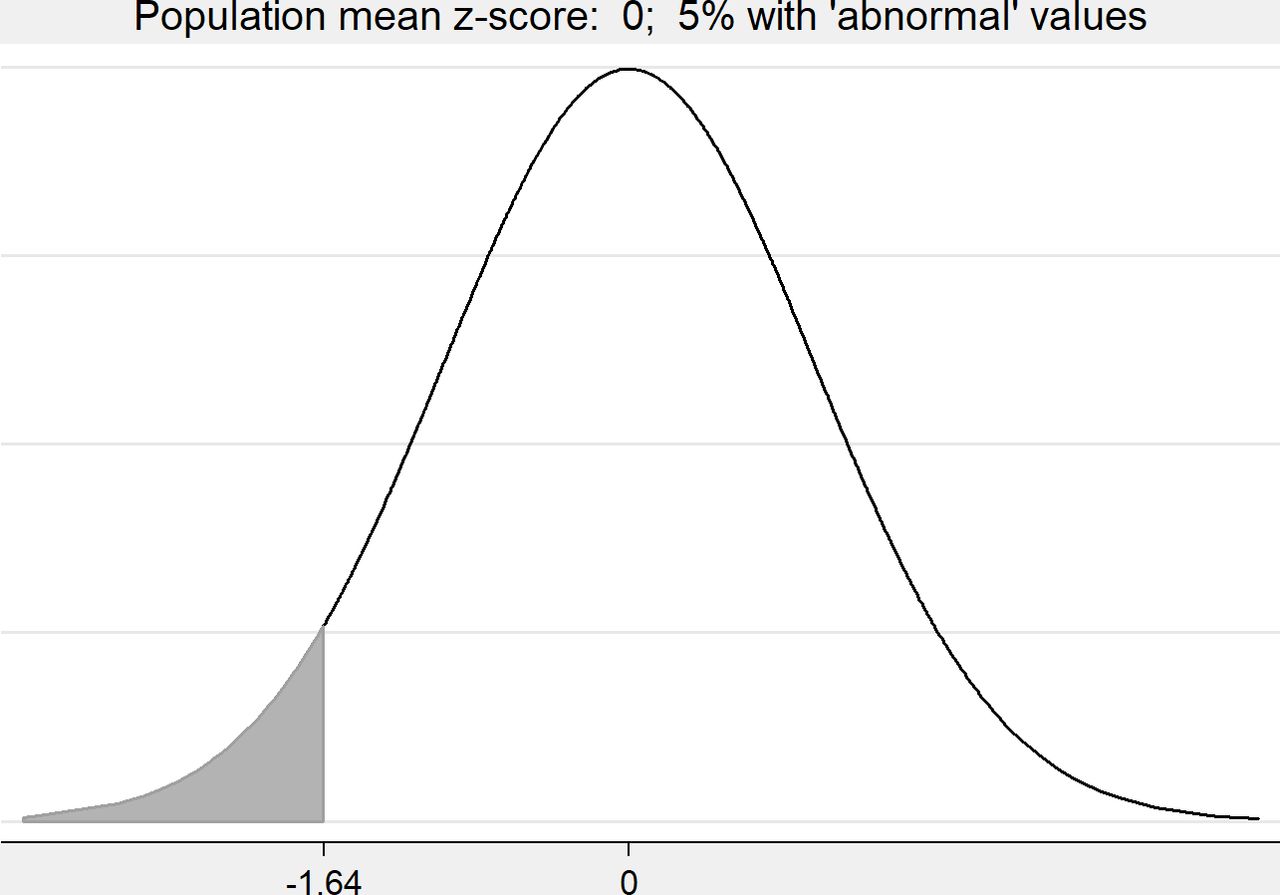
Hypothetical distribution showing the percentage abnormal (z< -1.64) with population mean=0.
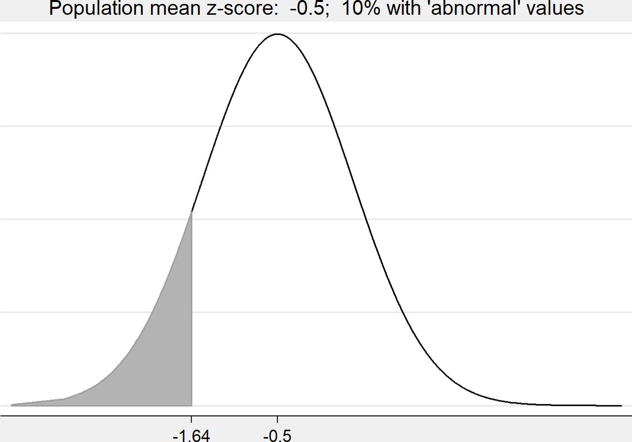
Hypothetical distribution showing the percentage abnormal (z< -1.64) with population mean=−0.5.

Hypothetical distribution showing the percentage abnormal (z< -1.64) with population mean=−1.
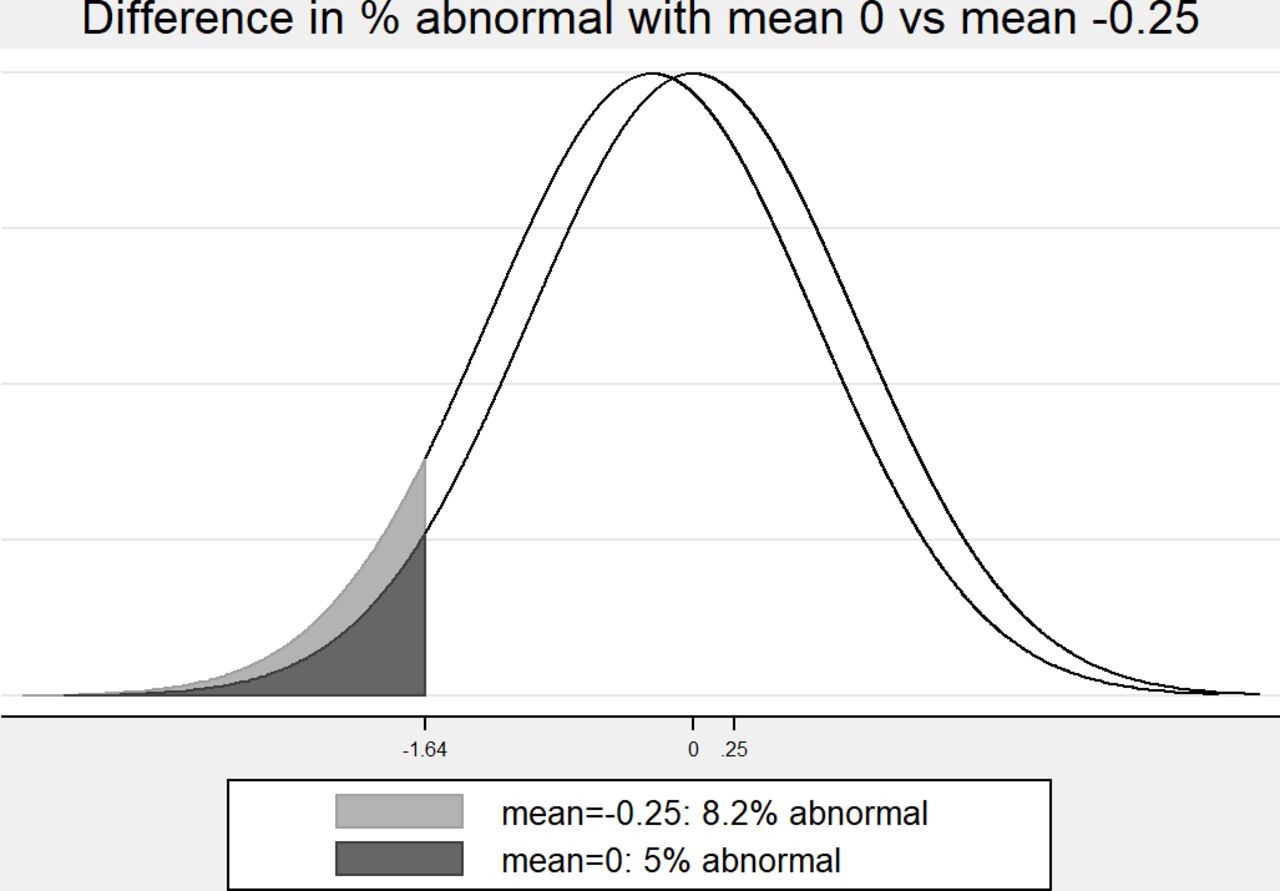
We now consider lung function z-scores in three populations that are Normally distributed with means 0 (general population), −0.5 (moderately vulnerable) and −1 (vulnerable) and compare each with another three populations that have means that are 0.25 lower (figures 4–6 and table 1). The fifth centile (z< -1.64) is used to define ‘abnormal’ and the difference is expressed as percentage points. We see that the percentage abnormal is affected by the means of the pairs of populations even though the difference in means is 0.25 in each case. Where the pairs of means are 0 and −0.25, the difference in the percentage abnormal is 3.2 percentage points (figure 4), for populations with means −0.5 and −0.75, the difference is 6.0 percentage points (figure 5), and for means −1 and −1.25 it rises to 8.7 percentage points (figure 6 and table 1). In other words, the same effect size, 0.25, has different consequences in different populations, so that a small difference in means has a greater impact in vulnerable populations. These results are tabulated in table 1.
Illustration of the effect of a small difference in mean (0.25 z-scores) in different populations using the fifth centile for a general population to define abnormal

Two hypothetical distributions with means 0 and −0.25 showing the difference in percentage abnormal (z< -1.64) between the two populations.

Two hypothetical distributions with means −0.5 and −0.75 showing the difference in percentage abnormal (z< -1.64) between the two populations.

Two hypothetical distributions with means −1 and −1.25 showing the difference in percentage abnormal (z< -1.64) between the two populations.
Real study example: United Kingdom Oscillation Study (UKOS)
The UKOS was a multicentre randomised controlled trial that compared outcomes in extremely premature babies allocated to either conventional mechanical ventilation (CV) or to high frequency oscillation (HFO) at birth. The trial found no evidence for any differences in respiratory or neurological outcome at hospital discharge or at follow-up at age 1 year or age 2 years.10–12 The ex-preterm children were followed up at age 11–14 years to explore possible effects of ventilation at birth on lung function in adolescence; a small but statistically significant difference was found in mean lung function z-score for the primary outcome, forced expiratory flow at 75% of forced vital capacity, and for the majority of secondary lung function outcomes, all in favour of HFO.13 This finding was in keeping with limited non-randomised evidence but the small effect size alongside a difference in mean z-scores was challenging to interpret clinically. We, therefore, calculated the difference in the proportion of patients with abnormal values using the fifth centile as the lower limit of normal (z< -1.64), which showed that the mean difference of 0.23 z-scores corresponds to a difference of 8.2 percentage points in the percentage of children with abnormal lung function (table 2). This relatively large difference arises because the populations were vulnerable prematurely-born children with mean lung function z-scores around −1.0. The clinical relevance of the percentages abnormal is more apparent than the means of lung function scores, since abnormal lung function in childhood is associated with poor respiratory health in adulthood.
Interpretation of results using the two approaches for high frequency oscillation (HFO) and conventional mechanical ventilation (CV)
Tools to help
We have shown with hypothetical and real data that a given effect size expressed as a difference in means, has different clinical implications in vulnerable populations compared with healthy populations. It is therefore helpful to report not only the difference in means but also the difference in the proportions (or percentages) of patients with abnormal values. In addition, it follows that when designing studies with two groups and a continuous outcome, it is important to consider the difference in the proportion abnormal as well as the difference in means when deciding on the appropriate MCID. In the next sections, we describe how to calculate the difference in proportions efficiently and how to incorporate these ideas into the calculation of sample size for a new study.
Calculation of the difference in proportions with abnormal values
In the example above (table 2), we did not calculate the proportion with abnormal measurements by dichotomisation using the usual formula, number abnormal divided by the total number. Instead, we have used the distributional approach14–18 to estimate the proportions and their difference. This methodology allows the difference in the proportions of individuals with abnormal measurements to be estimated with the same precision as the original analysis conducted with the mean z-scores, but without the usual loss in power associated with dichotomisation. A fuller description of the distributional approach methodology is given in online supplemental S1 with a full list of associated publications. Software is available in Stata19 and R (https://cran.r-project.org/web/packages/distdichoR/index.html).
Supplemental material
Calculation of sample sizes for study design
When deciding on the sample size for a new study, the issues described in this paper are particularly important if we are studying vulnerable patient populations. We need to ensure that the sample size is adequate to detect the minimum meaningful difference in the proportions of patients with abnormal values (eg, below fifth centile). In brief the following steps are needed:
Assume that the ‘control’ or normative population mean and SD are known and that the distribution is approximately Normal or can be transformed to Normal (as commonly assumed in many power calculations).
Identify the MCID for proportions, ‘MCIDprop’, from the proportion abnormal in the control population and the minimum meaningful difference as described above.
Compute the equivalent difference in means given the anticipated control population mean and SD, ‘MCIDmeans’ using standard formulae relating the mean and SD to the proportion beyond a given cut-point in a Normal distribution.
Calculate the target sample size based on the MCIDmeans.
In online supplemental, we have provided illustrative tables for z-scores (S2–S4) that allow researchers to estimate differences in the percentages with abnormal values for a range of mean population z-score values. In this way, researchers designing studies can explore the potential effect sizes for percentages at risk associated with a range of differences in mean z-scores and so make more informed decisions at the study design stage or when analysing an existing dataset where the sample size is fixed. By following this approach, it should be less likely that real differences will be missed or dismissed as clinically unimportant. The principles and calculations can easily be applied to other continuous variables where a cut-point can be used to define an abnormal value.
Discussion
In this paper, we have discussed the interpretation of difference in means in terms of the difference in percentages of individuals with abnormal values and we have shown that specific differences in means may have a different clinical importance depending on the patient population. There is an implicit recognition of this in Make et al’s paper where they give specific MCIDs for various outcomes relevant to patients with COPD.4 They suggest that 100 mL is a reasonable MCID for FEV1 They do not specifically discuss FEV z-scores. Similarly Jones et al20 discuss MCIDs for a range of COPD outcomes including lung function and while they do not discuss z-scores either, they acknowledge that baseline FEVR1R in a patient affects the degree of possible response so that a cross-the-board absolute value for MCID may not be appropriate. A Health Technology Review and associated papers helpfully explored in depth the methods used to specify the target difference for randomised trials but they did not discuss whether the MCID is constant across all populations.21–23
We have estimated the percentage (proportion) of patients with abnormal measurements using the distributional approach, which has the advantage that the whole distribution of data is used. Therefore, statistical power is not lost as it usually is when we dichotomise,14–18 and the comparison of means and percentages are estimated with the same precision. Thus, this dual approach addresses the difficulty in interpreting means, uses a method that is statistically robust, and provides estimates that are clinically meaningful.
We emphasise that we are not advocating replacing means with percentages or proportions alone. This would discard a substantial amount of information. Means must be computed, reported and interpreted, and where helpful, alongside the equivalent percentages of patients with abnormal values. Means, difference in means and difference in percentages should be presented with confidence intervals.
Using the distributional approach has a further benefit—it avoids the difficulty of multiple testing when both differences in means and differences in percentages are reported as the main outcome. Since the difference in percentages is a function of the difference in means, the two estimated differences provide equivalent inferences—they are alternative ways of presenting the same data in the same way, just as data from a 2×2 Chi-squared test can be presented as a difference in proportions and/or a ratio of proportions.
Limitations of our paper include that we have presented only one real-world example to keep the report short. While the example given is easily generalisable, further examples would be useful and we are planning future work that will illustrate the specific impact of these issues in a range of real-world situations. We also note that differences in means may be clinically meaningful such as when a study observes a large difference in means that has clear clinical importance.
In conclusion, we recommend that new studies using a continuous outcome where a cut-point may be used to define an abnormal measurement consider carefully what size of difference would be clinically meaningful in their population and to calculate both means and the percentage with abnormal values using an appropriate cut-point. This is particularly important in vulnerable populations. We recommend using the distributional approach to calculate the difference in percentages, since it retains statistical power and avoid issues with multiple testing. The researcher gets two-for-the-price-of-one.
Ethics statements
Patient consent for publication
References
Supplementary materials
Supplementary Data
This web only file has been produced by the BMJ Publishing Group from an electronic file supplied by the author(s) and has not been edited for content.
Footnotes
Contributors JLP and OS conceived this study and initiated a discussion with the other authors. JL conducted the brief descriptive review and contributed to the analysis. All authors, JLP, JL, JRR and OS, contributed to the interpretation of the results and to the drafting of the manuscript. All authors agreed the final submission.
Funding The authors have not declared a specific grant for this research from any funding agency in the public, commercial or not-for-profit sectors.
Competing interests None declared.
Provenance and peer review Not commissioned; externally peer reviewed.
Supplemental material This content has been supplied by the author(s). It has not been vetted by BMJ Publishing Group Limited (BMJ) and may not have been peer-reviewed. Any opinions or recommendations discussed are solely those of the author(s) and are not endorsed by BMJ. BMJ disclaims all liability and responsibility arising from any reliance placed on the content. Where the content includes any translated material, BMJ does not warrant the accuracy and reliability of the translations (including but not limited to local regulations, clinical guidelines, terminology, drug names and drug dosages), and is not responsible for any error and/or omissions arising from translation and adaptation or otherwise.