All or none exposure

The exposed and unexposed categories are denoted by 1 and 0 and the ratio of the event rates in these two categories as RR: 1.

FORMULAS

Classic (Levin) structure for AF_p, based on distribution of exposure in population

Denote by PF₁ the proportion (or fraction) of the total population time in the exposed category, and by PF₀the proportion in the unexposed category. The most popular1 11 16-18 formula for AF_p is Levin's original version. Levin began by defining the AF_p: its denominator is the rate (or number of cases) in the overall population, and its numerator is the difference between this and the one that would prevail if all of the person time were in the unexposed category. From this, he algebraically derived the estimating formula

Attributable fractions for specific exposure categories.

The case-based version uses as one of its inputs the “attributable fraction in the exposed”, namely

This is a specific AF, as it restricts attention to exposed cases. To emphasise this specificity, we label it AF₁. The under-appreciated fact that the “attributable fraction in theunexposed” is 0 becomes important later, and so we label the AF specific to cases in that category as AF₀ = 0.

(Miettinen) structure for AF_p, based on distribution of exposure in cases

The case-based version uses as its other input the number of exposed cases, expressed as a fraction of the overall number of cases. Denote this fraction as the “case fraction”,3CF₁. Then the case-based formula for AF_pis

or in the notation used here,

AF_p = AF₁ × CF₁.            [1C]

NUMERICAL EXAMPLE

Suppose, as is depicted in figure 1, that PF₁ = 2/5th of the population time (PT) is in the exposed category. Although the AF_p involves relative rather than absolute rates, suppose—for concreteness—that the event rates in the exposed and unexposed categories are 1.5 and 1.0 cases per 10⁴ PT units, so that the RR = 1.5, and the rate difference = 0.5 cases per 10⁴ PT units. Suppose further that the total population time is 10⁶ PT units.

• Download figure
• Open in new tab
• Download powerpoint

Figure 1

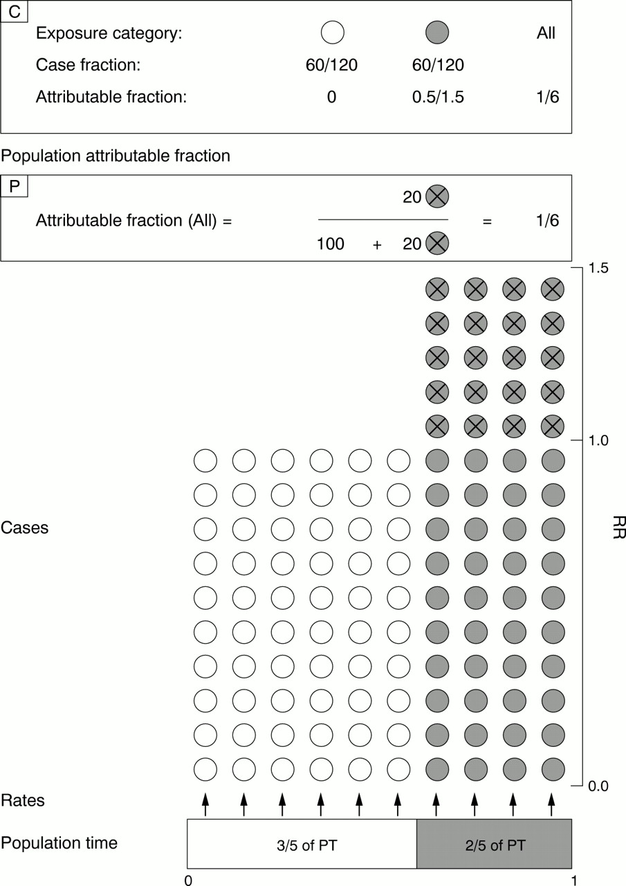
Population (that is, “overall”) attributable fraction (AF_p) when exposure is all(1) or none(0), based on distribution of exposure in population (P) and in cases (C).

 The PF₀ = 3/5th of the population time (PT) in the unexposed category is shown in white at the bottom of the diagram, and the PF₁ = 2/5th of the population time (PT) in the exposed category is shown shaded. Relative rates in these categories are RR=1 and 1.5. The corresponding numbers of cases arising from the two exposure categories are shown as white and shaded circles. The number of “excess” cases is depicted as shaded circles marked with an “X” (for “excess”).

 In the classic AF_p structure (summarised in inset “P”, with numbers of cases scaled up by 100), the total number of cases is divided into the lower (square) array denoting the number of expected cases (circles without an “X”, irrespective of exposure category) and the upper rectangular array denoting the number of excess cases. As the square array of “expected” cases has a base of width 1, and a height of RR = 1, it has an area of 1, representing one expected case. With these relative horizontal and vertical scales, the rectangle of excess cases has a base of PF₁ = 2/5 and a height of RR—1 = 1.5—1 = 0.5, so that its area (the “number of excess cases per 1 expected case”) is (RR—1) × PF₁ = 0.5 × 2/5 = 0.2. This 0.2 is 1/6th of the overall total of 1.2 cases.

 In the case-based AF_p structure (summarised in inset “C”), the total number of cases is divided first by exposure category. None of the unexposed cases (white circles) are “excess” cases. Of the exposed cases (shaded circles, constituting 1/2 of all cases), only a fraction represent excess cases. As 1 of every 1.5 exposed cases is “expected”, some 0.5 of the 1.5, or 1/3rd, are excess. Thus, 1/3 of 1/2 = 1/6 of all cases are excess cases.

Substitution of PF₁ = 2/5 and RR—1 = 0.5 into formula [1P] yields

THE NUMBERS AND STRUCTURES BEHIND THE FORMULAS

Conceptually, the Levin formula directly divides the total number of cases into “expected” cases—those that would occur even if all of the PT were in the unexposed category—and “excess” cases. With a total of 10⁶ units of PT, there are 10⁶ × (1.0 × 10^–4) = 100 “expected” cases. Some 2/5th of the overall 10⁶ PT units are in the exposed category, where the excess rate is 0.5 per 10⁴ PT units. The product of this PT and the excess rate in this category is 20 “excess” cases. These 20 represent 1/6th of the overall total of 100 + 20 = 120 cases. Note that the 20 can also be represented as the “observed−expected” number, while the 120 represent the “observed” number, in keeping with the structure in Miettinen's 1985 text (page 254–256),3 and Levin's2original conceptualisation.

The case-based formula begins with the same total of 120 cases and immediately “rules out” all unexposed cases, as, by definition, none of them are “excess” cases. Based on the amount of unexposed PT, they number 60, or 3/5th of the 100 “expected” cases discussed above. This leaves 60 exposed cases (1/2 of the overall total); if RR > 1 and finite, then only a fraction of these 60 exposed cases (or of the 1/2) are excess cases (that is, the maximum possible AF_p is 1/2). What fraction of these 60 represent excess cases? The RR=1.5 implies that of every 1.5 exposed cases, 1 is “expected”, while 0.5 of the 1.5, or 1/3rd, are excess. Thus, of the subtotal of exposed 60 cases, 20 are “excess” cases. As the subtotal of 60 exposed cases constitute 1/2 of all cases, and as only 1/3rd of the 60 are excess, then 1/3rd of 1/2, that is, 1/6 of all cases are excess cases. This 1/6th is thus a “fraction of a fraction”. The one fraction (1/2) is simply what fraction of all cases are exposed cases—which we have denoted by CF₁. The other, RR—1 as a fraction of RR, that is, 1/3, is the AF specific to the exposed category, namely AF₁.

THESE NUMBERS AND FORMULAS REPRESENTED PICTORIALLY

Figure 1 begins “at the base” with the denominators—the PT distribution—that generated the cases. Some 3/5th (= PF₀) of the PT are in the unexposed category (empty area) and 2/5th (= PF₁) are in the exposed category (shaded area). The cases that arise from these are represented by empty or shaded circles respectively; “excess” cases are marked with an “X” (for “excess”), while “expected” cases are not.

The number of excess cases as a fraction of all cases can be seen from two different views. In the first (Levin), the total number of cases is directly subdivided into two arrays—the (bottom) square array of expected cases, and the (upper) rectangular array of excess cases. With its height (representing the rate in category 0) arbitrarily scaled to 1, and with its entire base of 1, the square array of “expected” cases has an area of 1, representing one expected case. The width of the rectangle of excess cases is PF₁ = 2/5 and its height is RR—1 = 1.5—1 = 0.5, so that its area (the number of “excess cases per one expected case”) is (RR—1) × PF₁ = 0.5 × 2/5 = 0.2, yielding AF_p = 0.2/(1 + 0.2) = 0.2/1.2 = 1/6.

In the other view (Miettinen), the total number of cases is first subdivided into two arrays (and thus “case-fractions”) on the basis of exposure. Only the exposed (shaded) cases (a fraction CF₁ of all cases) are “eligible” to be excess cases. These exposed cases are then further subdivided into subarrays of excess and expected cases, yielding the attributable fraction AF₁ specific to the exposed cases. An attraction of this “fraction of a fraction” structure of the overall AF_pis that it does not explicitly involve the 3/5 : 2/5 exposure distribution in the source PT—a distribution that is not always easy to estimate—but rather the 60:60 split of the cases themselves.

For those who prefer algebra to pictures, an algebraic derivation of the case-based formula is given in the .

POPULATION ATTRIBUTABLE FRACTION AS A WEIGHTED AVERAGE

Unfortunately, immediately “eliminating” the unexposed cases, and focusing on the exposed ones, distracts from the fact that the case-based AF_p can also be viewed as a weighted average of the two category specific attributable fractions AF₀(= 0) and AF₁. Naturally, as the focus is on all cases, the weights are given by the relative numbers of cases in exposure categories 0 and 1—that is, by the proportions CF₀ and CF₁. Thus the weighted average of the two category specific fractions AF₀ and AF₁ across both categories of cases is 0 × CF₀ + AF₁ × CF₁ = AF₁ × CF₁. This representation of AF_p as a weighted average3 is key to understanding the case-based formula for the polytomous exposure situation considered next.

Polytomous exposure

Figure 2 depicts the data, and illustrates the correct AF_p calculations, for the “three exposure levels” example given in table 1.

• Download figure
• Open in new tab
• Download powerpoint

Figure 2

Population (that is, “overall”) attributable fraction (AF_p) when exposure is trichotomous, based on distribution of exposure in population (P) and in cases (C). Data are from table 1.

 The PF₀ = 5/10th, PF₁ = 3/10th, and PF₂ = 2/10th of the population time (PT) in the low, moderate, and high exposure categories are shown at the bottom of the diagram using increasing levels of shading. Relative rates in these categories are RR₀ = 1, RR₁ = 1.4 and RR₂ = 1.7. The numbers of cases arising from the three categories are shown as correspondingly shaded circles. The number of “excess” cases in each category is depicted as circles marked with an “X” (for “excess”).

 In the classic AF_p structure (summarised in inset “P”, with numbers of cases scaled up by 100), the total number of cases is divided into the lower (square) array denoting the number of expected cases (circles without an “X”, irrespective of exposure category) and the two (upper) rectangular arrays denoting the numbers of excess cases.

 In the case-based AF_p structure (summarised in inset “C”), the total number of cases is divided first by exposure category—CF₀ = 50/126, CF₁ = 42/126 and CF₂ = 34/126. None of those occurring in the lowest risk category (white circles) are “excess” cases, while 4/14th and 7/17th of the fractions in the higher risk categories are. Thus, 4/14th of 42/126 + 7/17th of 34/126 = 20.6% of all cases are excess cases.

CLASSIC STRUCTURE, BASED ON DISTRIBUTION OF EXPOSURE IN POPULATION

Again, the expected cases are shown in the square array of unmarked circles. Now, there are two sets of excess cases, denoted by the lightly shaded and more heavily shaded rectangular arrays of cases marked with an “X”. The scaled heights, {RR₁—1} and {RR₂—1}, of these rectangles, multiplied by their widths, PF₁ and PF₂ , yield excess “areas” of {RR₁—1} × PF₁ and {RR₂—1} × PF₂ respectively. These products represent the number of excess cases for every one “expected”. This “expected” versus “excess” partition of the cases leads immediately to the formula

For every one expected case, there are 0.12 + 0.14 = 0.26 “excess” cases, yielding an AF_p of 0.26/1.26 = 20.6% (last column of table 1). Note that applying formula 1P [all or none exposure] twice13 (second last column of table 1), overestimates the overall fraction of excess cases.

STRUCTURE BASED ON DISTRIBUTION OF EXPOSURE IN CASES

In this view, the AF_p is a sum of 2 “fractions of fractions”, that is,

as originally given in reference 3. As AF₀=0, the AF_p can also be seen as a weighted average of the category specific AFs over all 3 levels 0, 1 and 2

AF_p = CF₀ × AF₀ + CF₁× AF₁ + CF₂ × AF₂[2C']

For the data in table 1 and figure 2, the appropriate calculation is

(50/126) × 0 + (42/126) × (0.4/1.4) + (34/126) × (0.7/1.7),

yielding the “CF weighed” average, AF_p = 20.6%.

The explains a version that is useful when there are several strata or covariate patterns.

EFFECT OF COLLAPSING CATEGORIES OF HIGHER RISK INTO ONE

Several authors have noted11 19 20 or shown7 that the AF_p involving an exposure with levels 0, 1, ..., k is the same as if one first combined categories 1 to k and used the formula for the “all or none” situation. This is easy to see from figure 2, where the RR for the “moderate or high” category, relative to low, is 1.52, and PF_{moderate/high} = 0.5. Thus, for every one expected case, there are 0.5 × 0.52 = 0.26 excess cases, yielding AF_p = 0.26/1.26 = 20.6%.

The “distributive”21 property of the AF_pis useful in multiple regression if, instead of aggregating exposure categories, one subdivides them, to the point that each case defines its own exposure category. Details are given in the .

Stratified data

To correctly understand how to aggregate stratum specific AF_ps, first write

Then, with Σ denoting summation over the strata that form the aggregate, dis-aggregate the numbers of cases so that

Finally, rewrite this as

that is, as a weighted average of stratum specific AF_ps, with the numbers of cases in the each stratum as weights.

Figure 3 illustrates the correct calculation. Whether one arrives at the stratum specific AF_ps “by P or by C”, one must average them using the stratum specific numbers (or proportions) of cases as weights. The figure also illustrates the commonly used, but incorrect practice of coupling adjusted (RR-1)s with the marginal distribution of exposure in the overall source.

• Download figure
• Open in new tab
• Download powerpoint

Figure 3

Incorrect and correct calcuation of population attributable fraction in presence of confounding factor (hypothetical data).

Discussion

The primary aim of this article is to promote understanding of the AF_p formulas for a polytomous exposure, and for stratified data. To this end, you must begin with the simpler and more familiar, but not fully understood, representations for an all or none exposure. The article also shows how the two seemingly very different representations can both be derived—without algebraic manipulations—directly from the same diagram. A third aim is to increase awareness of the case-based formulas.

There are a number of possible explanations for the limited awareness and understanding of the case-based formulas. Some textbooks focus on the overall AF before (or without ever) dealing with the specific AFs that are aggregated to create the overall AF. Also, the case-based formula is given in fewer textbooks, usually without a complete derivation. The usually cited source3 does not explicitly derive it; instead it cites another source,22 which in turn cites an unpublished source. It was acknowledged (page 331)3 that the basis for the formula “may not be immediately obvious” and a cryptic explanation was offered. The “fraction of a fraction” formula is derived 11 years later (equation A.2.17, page 256)10 but in a seemingly different context, and using a purely algebraic manoeuvre that does not reveal the logic behind it (see ). The lengthy way in which the formula continues to be algebraically derived in subsequent articles and textbooks4 5 7 11 23 suggests that the simplicity and “immediate obviousness” of its structure have not been fully or widely understood.

The most important practical benefit of the case-based version is AF_p estimation from stratified, or individually matched, case-control studies22 where the classic formula is inappropriate.19 24 25 Variations on this version (see) are also increasingly used to derive—and quantify the sampling variability of—estimators of AF_p from stratified data or multiple logistic regression.4-8

The case-based structure also has conceptual benefits. Firstly, it emphasises that AFs refer to cases, and that the observed numbers of cases are the denominators of these AFs. This is in contrast with most epidemiological calculations, where numbers of cases serve as the numerators of statistics. As exemplified in figure 3, this difference has important implications for how to correctly aggregate stratum specific AF_ps—no matter which version of the formula (classic or case-based) is used to calculate the stratum specific AF_ps. Failure to appreciate this focus on cases may explain why authors, such as those of reference 13, incorrectly couple adjusted (RR-1)s with the marginal distribution of exposure in the source via formulas [1P] and [2P]. This is a common mistake.14 It is of note, and testimony to the naturalness of the case-based representation, that in the example in figure 3, the weighted average of the stratum specific AF_ps (the AF_ps having been derived from adjusted RRs), using the stratum specific numbers (or proportions) of cases as weights, yields the correct AF_pfor the aggregate.

Secondly, although originally derived for empirical estimates from case-control studies, the versatility of the case-based representation can be used in a broader context—for example, to structure the very AF_p parameter itself.3 8 (section 2, page 866). For these practical and conceptual reasons, the case-based representation needs to be better understood, and not presented in textbooks and articles simply as an algebraic fact.

Greater awareness and understanding of the formulas for polytomous exposure should also decrease computational errors. Even in the absence of confounding, the repeated application of formula [1P], once for each exposure category separately13 yields an overestimate of AF_p. As is made obvious by figure 2, a single application of formula [2P] yields the correct estimate.

Although its purpose was “multivariate” from the outset, the paper by Eide and Gefeller26 uses a graphical depiction similar to that presented here. It is helpful to think all of the covariate patterns shown in figure 1 of the Eide and Gefeller article as different levels of a single composite factor, in the spirit of the single polytomous factor in figure 2 of the present article.

The heuristic approach also gives insights into more realistic, and more complex, scenarios than are discussed in introductory textbooks. Indeed, it was questions from a colleague, in a study involving four levels of risk, and the consequences of switching, not to the lowest risk category, but to lower risk categories, that prompted the author to produce diagrams similar to figure 2. Readers are referred elsewhere10 (appendix 2.3, page 254–6)12 27 28 for more on this topic.

Technical details on estimating AFp from regression models can be found in papers by Benichou7 and Greenland and Dresher (page 1763).8 Benichou warns that his method for calculating the precision of the estimates is “complex”. The methods used by Greenland and Dresher are more tractable, but the matrix notation and associated calculations may still require the help of a statistician. The portion of the article by Ojaet al 29 that deals with conventional logistic regression modelling, and in particular the hand workable example in the , is a useful point of departure before tackling either of these papers. If you wish to avoid matrix calculations, then bootstrap confidence intervals are an attractive alternative.30