Article Text

Abstract
Objectives This paper looks into the socioeconomic determinants of risk of harmful alcohol drinking and of the transitions between risk categories over time among the population aged 50 or over in England.
Setting Community-dwellers across England.
Participants Respondents to the English Longitudinal Survey of Ageing, waves 4 and 5.
Results (Confidence level at 95% or higher, except when stated):
▸ Higher risk drinking falls with age and there is a non-linear association between age and risk for men, peaking in their mid-60s.
▸ Retirement and income are positively associated with a higher risk for women but not for men.
▸ Education and smoking are positively associated for both sexes.
▸ Loneliness and depression are not associated.
▸ Caring responsibilities reduce risk among women.
▸ Single, separated or divorced men show a greater risk of harmful drinking (at 10% confidence level).
▸ For women, being younger and having a higher income at baseline increase the probability of becoming a higher risk alcohol drinker over time.
▸ For men, not eating healthily, being younger and having a higher income increase the probability of becoming a higher risk alcohol drinker. Furthermore, the presence of children living in the household, being lonely, being older and having a lower income are associated with ceasing to be a higher risk alcohol drinker over time.
Conclusions Several socioeconomic factors found to be associated with high-risk alcohol consumption behaviour among older people would align with those promoted by the ‘successful ageing’ policy framework.
- EPIDEMIOLOGY
- GERIATRIC MEDICINE
- PUBLIC HEALTH
This is an Open Access article distributed in accordance with the Creative Commons Attribution Non Commercial (CC BY-NC 4.0) license, which permits others to distribute, remix, adapt, build upon this work non-commercially, and license their derivative works on different terms, provided the original work is properly cited and the use is non-commercial. See: http://creativecommons.org/licenses/by-nc/4.0/
Statistics from Altmetric.com
Strengths and limitations of this study
Longitudinal analysis.
Transitions across risks of harmful alcohol drinking.
Representative sample of older people.
Possible cohort effects not accounted for.
No comparisons with the rest of the UK.
Introduction
This paper looks into the socioeconomic determinants of harmful alcohol drinking among the population aged 50 or over in England. It also investigates what may be driving transitions between risk categories over time.
Since the first study that examined alcohol consumption among older people living in the community,1 a large literature has developed–a summary of the early literature is found in;2 for present comprehensive updates of the main issues, see.3–5
A number of papers have examined specific aspects, including: general health consequences,6 quantity and frequency,7 measuring tools,8 attitudes,9 comorbidities,10 screening,11 economic cost,12 demand for health and social care services,13 mortality,14–17 etc. Besides, a sizeable literature has looked into the psychosocial determinants of both consumption and changes in risks over time. This paper contributes to the latter category: it investigates statistical associations between alcohol risk categories and transitions between them over time and psychosocial characteristics of the population aged 50 or over in England. It will not focus on the health, financial or psychosocial consequences of harmful drinking.
The structure of the paper is as follows. A brief description of the academic literature on the psychological and social drivers behind harmful drinking in later life is included in section 2. Section 3 presents the data and section 4 describes the statistical methods used. Sections 5 and 6 set out the results of the analysis of the determinants of harmful drinking and of its transitions over time, respectively. Section 7 concludes.
Determinants of harmful drinking in old age: a synopsis of the literature
A recent literature review of alcohol use and alcohol-use disorders among older adults in India reports significant statistical associations between alcohol consumption in old age and higher educational status, younger age, better health status, lower chronic morbidity, employment status, socioeconomic status, auditory/locomotor impairment and asthma.18
Some of these variables (eg, age, income, education and gender) have been consistently found to be associated with risk of harmful drinking and alcohol abusei in old age across the literature at least since the late 1980s,22 although some studies are based on such small samples23 that low statistical power may have affected the SEs and, consequently, the significance of the results. A study based on a sample large enough for statistical purposes found that age is not a significant predictor.24 Two recent papers also report significant findings among alcohol consumption and these four variables, as well as with other covariates: significant associations have been found between alcohol consumption and education, age, subjective health status and gender among the older population in Sweden;25 in turn, the following list of characteristics were reported to be associated with unhealthy drinking among older people in Belgium: age, gender, social contacts, education, health status and socioeconomic status.26
Similarly, the literature on transitions has identified some recurring associations, such as declining risk with advanced age.27 Using data from the USA,28 it was found that increasing alcohol consumption among the older population was more likely among the more affluent, better educated, whites, males, unmarried, less religious and those in better self-reported health. Furthermore, a longitudinal study with US data on people aged 53 and 64 years found that changes in drinking categories were associated with gender, health, education, adolescent IQ, income, lifetime history of alcohol-related problems, religious service attendance, depression, debt and changes in employment.29 A study into changes in alcohol consumption among people aged 55–76 in the USA found that they were associated with gender, ethnicity, smoking, use of substances to reduce tension and social connectedness (and whether their contacts approved of heavy drinking or not).30 More recently, a 10-year study of alcohol use transitions among men aged between 50 and 65 in the USA reported that the different trajectories of risk were associated with age, education, smoking, binge drinking, depression, pain and self-reported health.31
Some culturally relevant aspects have also been identified: for example, a study on change in drinking consumption among older people in Japan found that apart from gender, education, age and depression, a related factor is employment status: consumption tends to drop significantly with retirement, which the authors ascribed to the role of alcohol consumption in Japanese work culture.32 This paper used data from England where, along with the rest of the UK, drinking patterns are shifting towards a Nordic-European pattern, ‘characterised by non-daily drinking, irregular heavy and very heavy drinking episodes (such as during weekends and at festivities) and a higher level of acceptance of drunkenness in public’ (p. 11, ref. 33). Therefore, consideration needs to be given to its results as applicable to a particular cultural milieu with evolving drinking patterns.
Table 1 presents a summary of the main findings in the literature.
Main findings in the relevant literature
Data
This paper is based on data from the English Longitudinal Study of Ageing (ELSA), a longitudinal multidisciplinary data study from a representative sample of men and women aged 50 years and over living in private households in England.55 To study the determinants of harmful drinking, we used the latest wave (wave 5) of ELSA corresponding to the years 2010–2011 (sample size: 9251) and, for the transitions analysis, the last two waves (wave 4 corresponds to the years 2008–2009).
We defined risk of harmful drinking following the guidelines set out by the National Institute for Health and Care Excellence (NICE). NICE has defined the following levels of risk of harmful drinking:
Lower risk drinking: ≤21 units per week (adult men) or ≤14 units per week (adult women).
Increasing-risk drinking: 22≤50 units per week (adult men) or 15≤35 units per week (adult women).
Higher risk drinking: >50 alcohol units per week (adult men) or >35 units per week (adult women).
This definition is part of the classification adopted by NICE to set guidelines and public health guidance in England. See also.56 It is consistent with a 1995 report by the Department of Health on ‘sensible’ drinking,57 which had set daily but not weekly guidelines. Although it is not without problems, see58 ,59 for a discussion. Several hundred estimation measures and instruments, primarily designed as screening tools, are available (the most widely used include the Severity of Alcohol Dependence Questionnaire; the Alcohol Use Disorders Identification Test, the CAGE test, the Michigan Alcoholism Screening Test, the FAST alcohol screening test, etc).60 Furthermore, we carried out a sensitivity analysis and found that relatively minor changes in the cut-off points for higher risk drinking altered the significance of our regression results (see online supplementary annex 1).ii
Two additional considerations regarding the definitions of risk by NICE merit a comment here: the use of a weekly, instead of daily, guideline may mask episodic heavy drinking—a non-negligible and increasing issue among middle-aged people in England61 ,62—and the lack of specific guidelines for older people (eg, for people aged 65 or older) is problematic in the light of evidence on physiological and metabolic changes in alcohol absorption and effects associated with individual ageing,63 which led the Royal College of Psychiatrists to recommend reduced thresholds for older people.64
However, we have used this definition of risk given that this paper is based on English data and that one of the objectives of the paper is to inform and influence policymakers and practitioners in England who have to follow NICE guidelines.
The literature on alcohol abuse in old age distinguishes between people who consume low quantities of alcohol and abstainers.65–67 Our data do not allow us to make such a distinction, but we have separated those respondents who said they had not drunk any alcohol at all during the previous week from those who did. Therefore, in this paper, we have included a fourth risk category which we have termed the ‘abstainers’, but we emphasise that the individuals in this category may not necessarily be teetotallers but consistent infrequent drinkers,31 and therefore there may be some overlap between this group and the lower risk drinkers. Nevertheless, since in our models we focused on higher risk drinkers, this distinction between abstainers and lower risk drinkers is inconsequential for our results.
The literature has also introduced a distinction between early-onset and late-onset cases,68–70 as well as that between having a history of problem drinking or not.28 ,52 However, the data do not allow us to distinguish between early and late onsets or about individual lifetime alcohol consumption patterns, so the paper considers current abuse risk and changes across risk categories in relation to covariates measured at baseline with a disregard of alcohol ingestion patterns at early ages.
Finally, the literature that focuses on the relation between stressful life events and changes in alcohol consumption in old age distinguishes between events with short-term effects and those with long-term implications.71 In order to discern between short-term and long-term effects of life events, we would need data that covered longer than 2 years as in this paper; furthermore, we would also need data from years before the events took place to account for simultaneous causality and unobserved individual endogeneity;72 hence, we are not going to investigate whether this distinction holds for our sample.
ELSA contains questions about weekly consumption of spirits, wine and beer. In order to use NICE guidelines, we used the conversion tables in the ‘alcohol unit calculator’ produced by the National Health Service (NHS) to help find out how many units there are in the most popular glass sizes and measures in the country.iii According to this tool, 1 glass of wine is equivalent to 2.1 units, 1 pint of beer to 2.8 units and 1 measure of spirits to 1 unit.
Following the suggestions by one of the reviewers, we estimated the effect on our results of changing the conversion ratios for wine and beer. Thus, we calculated consumption according to the conversion measures introduced in 2007 to the General Lifestyle Survey (GLS):iv one pint of a normal strength beer is equivalent to 2 units, a 175 mL glass of wine is equivalent to 2 units and a 250 mL glass of wine is equivalent to 3 units. Furthermore, we also applied the conversion tables in the drinkaware website (http://www.drinkaware.co.uk): 1 glass of wine, equivalent to 3 units, and 1 pint of beer, equal to 3 units.
Table 2, the starting point for the transitions analysis, presents the data on risk for those respondents surveyed in both waves. It also presents the transitions using the two other alternative conversion measures;–the widest variations are found using the drinkaware definitions.
Alcohol consumption by risk—ELSA waves 4 and 5 alternative conversion measures
We included the following variables in our models:
Age
Income: equivalised household net income per week (truncated at 1 penny). The equivalisation was performed by the OECD equivalence scale. Income is imputed net of taxes, and there may be records with negative incomes due to, for example, self-employment losses. We set any negative incomes to one penny, but not exactly to zero as in,73 to allow the logarithmic transformation.
Education: we categorised this variable into four levels:
No Qualifications
NVQ1/CSE other grade equivalent
NVQ2/NVQ3/GCE A/GCE O Level or equivalent and Foreign
NVQ4/NVQ5/Degree or Higher education below degree
Smoking: number of cigarettes smoked per day
Physical activity: we categorised this variable into four levels:
Sedentary
Low
Moderate
High
Depression: whether the respondent felt depressed much of the time during the past week
Loneliness: four-item scale based on the 20-item Revised UCLA loneliness scale,74
How often do you feel you lack companionship?
How often do you feel isolated from others?
How often do you feel left out?
How often do you feel in tune with the people around you?
(For the first three questions, categorised as lonely if responded ‘some of the time’ or ‘often’; for the last question, if responded ‘hardly ever’ or ‘never’).
Self-reported health: categorised into Poor, Fair, Good, Very Good, Excellent
Ethnicity: whether respondent is white (=0) or not (=1)
Gender: Female=0; Male=1
Marital Status: three categories:
Single, legally separated, divorced
Married, first and only marriage, remarried, civil partner
Widowed
Caring responsibilities: whether respondent looked after anyone in the past week (=1) or not (=0)
Children in household: total number of children inside the household
Religion: how important religion is in the respondent’s daily life. Four levels:
Very important
Somewhat important
Not very important
Not at all important
We excluded this variable from the transitions section, because we detected potential errors in the categorisation of the questions about religion in wave 4.
Economic Activity: Three categories:
Employed
Inactive (including unemployed, due to the low number of cases)
Retired (including semiretired)
Social detachment: if detached in three or more of the following four domains. Source:75
Civic participation: Not a member of a political party, a trade union, an environmental group, a tenants’ or neighbourhood group or neighbourhood watch, a church or religious group, or a charitable association; and did not do voluntary work at least once in the past year.
Leisure activities: Not a member of an education, arts or music group or evening class, a social club, a sports club, gym or exercise class, or of another organisation, club or society.
Cultural engagement: neither went to a cinema, an art gallery, a museum, a theatre or a concert nor to an opera performance at least once in the past year.
Social networks: Do not have any friends, children or other immediate family or if they have friends, children or other immediate family, have contact with all of them (meeting, phoning or writing) less than once a week.
Healthy diet: whether respondent consumes five or more portions of vegetables (excluding potatoes) or fruit a day
Table 3 presents the descriptive statistics for each variable for wave 5.
Descriptive statistics—wave 5
For wave 5, table 4 presents the distribution of the sample by risk category and gender and figure 1 presents the distribution of consumption of alcohol units (excluding abstainers) by gender. We notice the largest gender discrepancy among abstainers: 64% of abstainers are women; besides, 50% of women are abstainers (against 34% of men).
Distribution of sample by risk and gender wave 5

Distribution of respondents by number of alcohol units consumed.
Both table 4 and figure 1 suggest that we should run separate models for women and men, further confirmed by a χ2 test of independence applied to table 4: there is a significant statistical association between risk and gender (χ2=259.07, df=3, p value=0).
For the transition analysis, we used a balanced panel, that is, only respondents in both waves were included. This could in principle introduce bias if dropping out of the survey was to any extent contingent on drinking levels. Therefore, we checked for a significant association between attrition and consumption levelsv. To this purpose, we fitted an OLS regression with dropping out as the outcome variable on age (and age squared), gender, smoking, health status and alcohol consumption units. Alcohol consumption units are not significant. Further, we compared the statistical distributions of alcohol consumption units among respondents in wave 4 who took part in the survey in wave 5 and those who did not, for men and women separately, by means of the consistent univariate entropy density equality test bootstrapped with 100 replications.vi Again, we failed to find an association between alcohol consumption in wave 4 and attrition in wave 5.vii Therefore, our results would not suffer from ‘sick quitter’ bias. It is worth noting that studies of attrition by alcohol consumption patterns report inconsistent findings across waves. For example,77 the odds for dropping out at one wave was higher among respondents with high-alcohol intake, but that abstainers had increased odds for dropping out at other waves. Furthermore, a literature review78 failed to find any association between attrition and alcohol consumption levels.
Statistical methods
To identify variables associated with the probability of being or not being in the higher risk category, we used a logistic regression model. Given the small proportion of respondents in this category, we applied the Firth correction to account for any bias introduced by zero inflation.
We included age squared as a term in the regression models to account for any non-linearity in the association between age and risk.
Heavy drinking in old age is associated with short-term mortality;12 ,15 ,79–83 hence, the sample could suffer from an over-representation of moderate drinkers at higher ages as heavy drinkers might have died earlier. Therefore, we checked for this possible selection bias: given that this is a cross-sectional study and that the data do not include any information about past drinking behaviour, we ran models with age truncated at 70. We compared the results with those from the full sample but failed to find any significant differences, so preliminarily we can rule out the presence of selection bias in our sample. Comparing logistic models fitted on different groups or samples is not straightforward, and there is no one accepted method. We applied the heterogeneous choice model procedure,84 for which we fitted heteroscedastic binary response models via maximum likelihood and ran likelihood tests to compare both models (results can be requested from the author).
With regard to the transition analysis, we carried out a Markov chain model assuming continuous and homogeneous time fitted by maximum likelihood, with the same number of regressors as in the previous models (except religion, as indicated above). We used the package ‘msm’ in R.85
Markov chains are stochastic processes according to which, for each respondent, the risk of being in any one particular state in one wave depends solely on the state in which the person was in the previous wave, plus a number of characteristics observed also in the previous wave.86 ,87
We computed discrepancy scores88 for consumption of wine, spirits and beer and for the number of drinking days, for men and women separately, as the difference between units in waves 4 and 5. We failed to find any systematic or consistent patterns and the correlation coefficients between the discrepancy scores of each type of alcoholic drink and the number of drinking days were all very low (max=0.33, for consumption of beer and drinking days for women). Therefore, we can rule out inconsistency in the answers.
In this paper, we ran models for two and four states. The two-state models fitted transitions between being and not being in the higher risk category; the four-state models allowed for transitions across any of the four risk categories. However, owing to sample limitations, the four-state models could not be computed: with four states, none of them irreversible, there are 16 possible transitions, which proved too many for our samples. Consequently, we only report the results for the two-state models.
Our two-state models, shown separately for women and men, estimate the probability of a respondent becoming a higher risk alcohol drinker in wave 5, given that they were not a higher risk alcohol drinker in wave 4, and the probability of becoming a not at-higher risk alcohol drinker in wave 5, given they were a higher risk alcohol drinker in wave 4—conditional on a number of personal characteristics such as age, education attainment, marital status, etc—as measured in wave 4.
Results
Table 5 presents the statistical associations of the different covariates with the probability of being in the higher risk drinking category in wave 5. In other words, the table answers the research question ‘who would be more likely to be classified as a higher risk alcohol drinker’.
Wave 5—logistic regression results (Firth bias-corrected) probability of being in the higher risk drinking category (people aged 50 or over)
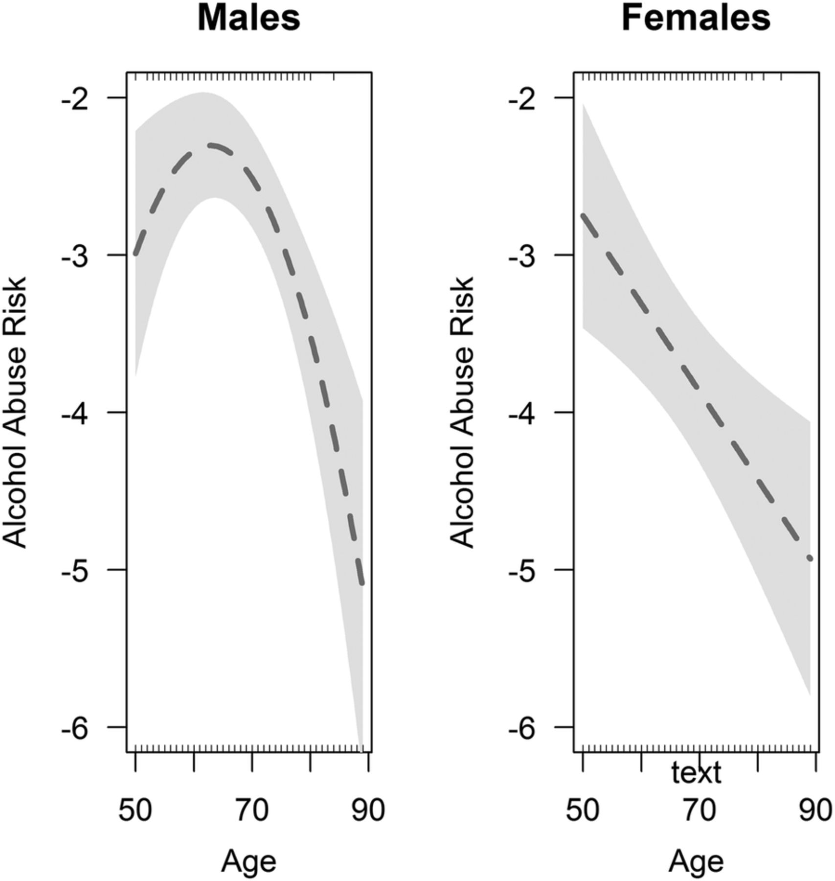
The probability of being in the higher risk drinking category decreases with age for men and women. Moreover, there is a non-linear association between age and risk for men, but not for women; hence, we reran the model for women with only a linear specification of the variable age–table 5 shows both sets of results. Figure 2 presents the probability of being in the higher risk drinking category by age conditional on all the other variables included in the model. The conditional probability plot in figure 2 shows that the risk for men becomes highest in the early 60s. For women, the conditional probability of drinking at harmful levels exhibits a linear negative slope with age. The non-linear association with age and the associated finding that, for men, the probability of being in the higher risk category peaks in the mid-60s could give empirical support to the hypothesis that current cohorts of older people are carrying on the relatively higher consumption levels they exhibited earlier on in their lives into older age compared to previous cohorts.61 However, we can only express the possibility here as we could not distinguish between age, cohort and period effects with the data under study to explore this hypothesis in full.
Conditional probability plot of being at higher risk drinking category by age and gender.
Income is positively associated with a higher risk for women but not for men, while the number of cigarettes consumed is positively associated for both sexes.
Reporting better health is positively associated with the probability of drinking at harmful levels.
Neither being depressed nor feeling lonely is associated with a higher risk of harmful drinking.
Higher risk drinking is more likely among white men, but ethnicity is not significant for women.
Having caring responsibilities reduces the probability of being at higher risk for women. Considering that their religion is very important for their lives is not significantly associated with the probability of being a higher risk drinker either for men or women.
Both for men and women, a higher risk is positively associated with higher educational attainment.
Economic activity is not significantly associated with risk, except retirement for females, which increases the likelihood of drinking at higher risk levels.
Single, separated or divorced men show a greater risk of harmful drinking.
None of the other variables included in the models presented statistically significant associations with risk.
Online supplementary figures A1 and A2 in annex 1 present a sensitivity analysis of the estimates in table 5 after modifying the threshold for higher risk from NICE guidelines. In turn, online supplementary figures A1 and A2 in annex 2 present the results using the alternative conversion tables. These sensitivity analyses show that alternative definitions of cut-off levels and conversion units do not introduce substantial changes to the results. Only coefficients significant at the 10% level present variations across the choices of thresholds and conversion units. By and large, our results are robust to these methodological changes.
It is important, once a model has been fitted, to estimate whether any predictions stemming from it can be validly extended to other samples or to the same participants in the future. This is known as the validation stage. Validation can be external or internal, that is, it can resort to data not used in the fitting of the model (external) or to the data included in the estimation stage (internal). We opted for an internal validation of our models, for which we applied the bootstrap method.88–90
Table 6 presents the tests of internal validation of the logistic regression models for men and women. The c-statistic measures the discriminative ability of the model: the concordance between predicted and observed responses. The slope statistic (also known as the shrinkage factor) is a measure of the amount of overfitting likely to be present.
Resampling validation of logistic models (bootstrap n=200)
The c-statistic ranges between 0.5 (no predictive discrimination) and 1 (perfect separation power between respondents with different harmful drinking risk levels). We note that the models discriminate slightly better among women than men, but in both cases we obtain acceptable concordance. With regard to the shrinkage factor, it should be of concern if the slope coefficient fell below 0.85.89 In our case, the results indicate a mild overfitting: about 11% (for women) and 13% (for men) of the model fit are statistical noise, that is, within acceptable levels.
Transitions
Table 7 presents the results for the Markov chain models, which estimate the associations between being or not being classified as a higher risk drinker in wave 4 and the risk classification in wave 5 conditional on a number of personal characteristics measured in wave 4. For completeness, it includes the results from the alternative conversion measures already described (ie, the drinkaware and the GLS measures).
Transitions between risks—wave 4 and wave 5—Markov chain models
For women who were not classified as higher risk drinkers in wave 4, our findings suggest that being lonely, being younger and having a higher income in wave 4 are all associated with a higher probability of becoming a higher risk alcohol drinker in wave 5. In turn, observing a healthy diet is associated with a lower probability of becoming a higher risk alcohol drinker. No variables were significantly associated with ceasing to be in the higher risk category by wave 5 for those women who were classified as such in wave 4.
For men who were not classified as at higher risk in wave 4, a higher probability of becoming a higher risk alcohol drinker in wave 5 is associated with not eating healthily, being younger and having a higher income. Furthermore, we also found that the presence of children living in the household, being lonely, being older and having a lower income increases the likelihood of ceasing to be at higher risk by wave 5. The last two findings are worth a further explanation: we found that, for men, the older they are, the less likely it is they may become higher risk drinkers, and for those at a higher risk category, the more likely it is that they may cease to be so. Similarly, for income levels, the higher the income, the more likely that men may become higher risk drinkers if they were not so, and the less likely that they cease to be higher risk drinkers if they happened to be classified as such.
Apart from the associations with covariates at baseline (ie, wave 4), we also investigated whether the transitions into and out of the higher risk category between both waves were associated with having been widowed, retired during this period, taken on caring responsibilities or the ‘empty nest’ syndrome (ie, if there were any children living in the household in wave 4 and they had all left by wave 5). We failed to find any significant associations (results can be requested from the author).
Comparing the results in tables 5 and 7 using alternative measures, we find that the changes in conversion units for wine and beer are more crucial to explain the factors associated with becoming a higher risk drinker over time (ie, transitions) than with those associated with drinking at harmful levels at one point in time. For example, when using the GLS conversion units, only three variables result significantly for the transition between not being at a higher risk to becoming a higher risk drinker among women and with the same signs as before—age, loneliness and income—while for men loneliness, age and income cease to be significantly associated with ceasing to be in a high-risk category. In turn, the drinkaware measures render solely age and healthy diet as significant variables regarding the transition into harmful levels for women.
A final methodological point has to do with under-reporting. A recent study,91 using data from the Health Survey of England (HSE), failed to find any association between under-reporting and age among people aged 50 or over. ELSA uses the same respondents as the HSE, and therefore we are confident that our results are not contaminated by under-reporting. However, that study found that under-reporting is probably more to do with the drinking pattern than demographic or social factors, which means that respondents classified as at higher risk might be under-reporting their consumption more than those drinking at safer levels.viii
Conclusions
Several socioeconomic factors are associated with high-risk alcohol consumption behaviour among older people, which must be factored in when designing and evaluating preventative interventions. Without repeating the findings discussed above, we can sketch—at the risk of much simplification—the problem of harmful alcohol drinking among people aged 50 or over in England as a middle-class phenomenon: people in better health, higher income, with higher educational attainment and socially more active are more likely to drink at harmful levels. This characterisation mirrors the main results from some studies among people of working age.92 ,93
Among the many policy frameworks around ageing, for example, ‘active ageing’,94 ‘productive ageing’,95 etc, ‘successful ageing’64 is one of the most widely used and embraces components such as non-smoking, greater physical activity, more social contacts, better self-rated health and absence of depression, among others.34 ,35
Alcohol consumption is growing among older people in England.36–39 The results reported in this paper allow us to conclude that, generally speaking, people aged 50 or over ageing ‘successfully’ in England are more at risk of drinking at harmful levels or of developing harmful drinking consumption patterns than those who fit less well into the paradigm of ageing ‘successfully’. There is some evidence that to some extent this is a generational trait: current age cohorts of older people exhibited higher alcohol consumption levels in the past and would be carrying on their relatively higher levels into older age compared to older people in the past.61 Nevertheless, our findings suggest that harmful drinking in later life is more prevalent among people who exhibit a lifestyle associated with affluence96 and with a ‘successful’ ageing process. Harmful drinking may then be a hidden97 health and social problem in otherwise successful older people. Consequently, and based on our results, we recommend the explicit incorporation of alcohol drinking levels and patterns into the successful ageing paradigm.
A number of limitations to this study need to be pointed out. First, we restricted the longitudinal study to two waves. A longer window would make the detection and analysis of trends possible. Second, the data set used in this paper, ELSA, although representative of people aged 50 or over in England, is carried out every 2 years. Consequently, the transitions analysed in the paper comprised changes between two points in time 2 years apart, which is an important gap to study lifestyle changes and consumption patterns of frequently purchased goods such as alcoholic drinks. Third, and also related to ELSA, we mentioned in the text that it is not possible to obtain scores for other scales and instruments; unfortunately, the survey only records weekly rather than daily consumption. Fourth, we restricted the main results to the definitions of risk by NICE although, as mentioned earlier, there is some merit in defining levels of risk specifically for older people based on available physiological evidence.
References
Supplementary materials
Press release
Press release
Files in this Data Supplement:
Footnotes
Funding This study was fully funded internally.
Competing interests None declared.
Ethics approval This is a secondary analysis of publicly available data. No ethical approval was required.
Provenance and peer review Not commissioned; externally peer reviewed.
Data sharing statement No additional data are available.
↵i Harmful drinking is defined as a pattern of psychoactive alcohol consumption causing health problems.19 ,20 In turn, alcohol abuse is akin to alcohol dependence, which is characterised “by craving, tolerance, a preoccupation with alcohol, and continued drinking in spite of harmful consequences” (p. 754, 21)
↵ii We are grateful to one of the reviewers for this suggestion.
↵iii See http://www.nhs.uk/Tools/Pages/Alcohol-unit-calculator.aspx. Retrieved on 6 February 2015.
↵iv General Lifestyle Survey 2011. Office for National Statistics 2013. Available at: http://www.ons.gov.uk/ons/rel/ghs/general-lifestyle-survey/2011/index.html
↵v We are grateful to one reviewer for highlighting this possibility.
↵vii Results available from the corresponding author.
↵viii We are grateful to Dr Sadie Boniface, Research Associate at UCL Epidemiology & Public Health, University College London, for this clarification in a personal communication.