Article Text

Abstract
Objective To determine a practical approach for deriving life expectancy estimates in Australian New South Wales local government areas which display a large diversity in population sizes.
Design Population-based study utilising mortality and estimated residential population data.
Setting 153 local government areas in New South Wales, Australia.
Outcome measures Key performance measures of Chiang II, Silcocks, adjusted Chiang II and Bayesian random effects model methodologies of life expectancy estimation including agreement analysis of life expectancy estimates and comparison of estimate SEs.
Results Chiang II and Silcocks methods produced almost identical life expectancy estimates across a large range of population sizes but calculation failures and excessively large SEs limited their use in small populations. A population of 25 000 or greater was required to estimate life expectancy with SE of 1 year or less using adjusted Chiang II (a composite of Chiang II and Silcocks methods). Data aggregation offered some remedy for extending the use of adjusted Chiang II in small populations but reduced estimate currency. A recently developed Bayesian random effects model utilising the correlation in mortality rates between genders, age groups and geographical areas markedly improved the precision of life expectancy estimates in small populations.
Conclusions We propose a hybrid approach for the calculation of life expectancy using the Bayesian random effects model in populations of 25 000 or lower permitting the precise derivation of life expectancy in small populations. In populations above 25 000, we propose the use of adjusted Chiang II to guard against violations of spatial correlation, to benefit from a widely accepted method that is simpler to communicate to local health authorities and where its slight inferior performance compared with the Bayesian approach is of minor practical significance.
- EPIDEMIOLOGY
- PUBLIC HEALTH
- Mortality
This is an Open Access article distributed in accordance with the Creative Commons Attribution Non Commercial (CC BY-NC 3.0) license, which permits others to distribute, remix, adapt, build upon this work non-commercially, and license their derivative works on different terms, provided the original work is properly cited and the use is non-commercial. See: http://creativecommons.org/licenses/by-nc/3.0/
Statistics from Altmetric.com
Strengths and limitations of this study
-
We explored the methods for estimating life expectancy in small and large populations and propose a hybrid approach for estimating life expectancy using adjusted Chiang II in populations larger than 25 000 and a Bayesian random effects model in populations of 25 000 or less for intended use by health administrators to support planning and policy.
-
Using a single of parameter of population size to decide on the method to use for life expectancy estimation is a simple criterion to follow and should be easily implemented by health agencies for the large scale production and processing of life expectancy estimates across administrative areas with widely varying population sizes.
-
The main limitation of the study is that the implementation of two methods for the derivation of life expectancy estimates, including the more complex Bayesian approach, could be difficult to communicate by health agencies.
Introduction
Life expectancy, the expected number of years of life remaining at a specified age (eg, at birth or at age 65 years), reflects the mortality experience of a population and can be used to assess potential health inequalities between geographical areas, evaluate the effectiveness of public health initiatives and contribute to the development of future healthcare policies. Accurate life expectancy estimation in small populations is also an important contributor to local population health indices which is central for health needs profiling and necessary to support the equitable and efficient planning and funding of clinical and public health services in local areas. A widely used technique for the calculation of life expectancy is the Chiang method which computes estimates using life tables,1 ,2 and is implemented by leading statistical agencies such as the WHO and the Office for National Statistics in the UK. A recent method described by Silcocks et al3 also calculates life expectancy using life tables but uses a different mathematical framework to calculate life expectancy and its variance. The Silcocks method was intended for application at subnational levels. A notable difference between the two methods is that Chiang assumes there is zero variance contributed by the final age interval as the probability of death is fixed at one whereas Silcocks calculates the variance based on the width of the final age interval.
Chiang and Silcocks methods provide robust and reliable life expectancy estimates in large populations. However, the results of the methods are less stable in small populations due to large SEs and become increasingly prone to calculation failures. Furthermore, several recent research reports showed that life table estimates increasingly overestimated (bias) life expectancy as population sizes fall below 5000 years of life at risk.4–7 As such, Toson and Barker4 and Eayres and Williams5 recommended that a minimum population size of 5000 is used for the calculation of life expectancy when using traditional methods. However, a recent study by Jonker et al7 proposed that life expectancy could be estimated in areas with populations as small as 2000 person-years at risk using Bayesian random effects models. Other studies have investigated ways to improve the estimation of life expectancy in small populations. A UK study explored methods of closing the life table in small populations to address the unusually high life expectancy measures that can occur when there are low numbers of deaths in the final age interval,8 and Bravo and Malta9 investigated the use of graduation models to smoothen crude mortality rates to augment the reliability of life expectancy estimates. However, these methods are limited by the absence of estimation methods for SEs and CIs, which are necessary for the comparison of estimates between different areas or to a reference standard. A simple and effective option to extend the use of traditional life expectancy methods in small populations is data aggregation which effectively augments the person years at risk. However, aggregation through time or across areas would limit the capacity of estimates to reflect current conditions or compromise area specificity.
The aim of this study was to investigate the methods available for the estimation of life expectancy across different administrative geographic boundaries. We compared Chiang II and Silcocks methods of life expectancy estimation and examined the limitations of these traditional methods in small populations. The performance of an adjusted Chiang II method modified to include the Silcocks method of calculating variance for the final age interval was also compared with a Bayesian random effects model of life expectancy estimation. The ultimate objective of this study was to decide on a practical solution to provide the best life expectancy estimation for subnational administrative areas that display diversity in population sizes and clearly present the approach for use by health agencies.
Methods
Population data, life expectancy estimation and agreement analysis
Australian Bureau of Statistics (ABS) mortality data and estimated residential population data over the period 1976–2007 for the 153 New South Wales (NSW) Local Government Areas (LGAs) were used for this study. The datasets were accessed through the NSW Ministry of Health's Secure Analytics for Population Health Research and Intelligence (SAPHaRI) system. Two traditional life table methods of calculating life expectancy, Chiang,1 ,2 and Silcocks,3 were investigated in addition to a third Bayesian random effects model of life expectancy.7 The Bayesian approach ‘borrows strength’ from the strong correlation in mortality rates between genders, adjacent age groups and geographical areas through the specification of multiple multivariate conditional autoregressive priors within the Bayesian framework. An assumption central to the method is that mortality rates might be spatially correlated and that intelligent Bayesian smoothing can improve the precision of estimated mortality rates for the derivation of life expectancy.10 On the other hand, the application of the method when the degree of spatial correlation is low or zero might lead to biased estimates.10 Full details of the Bayesian approach are provided in Jonker et al7. Briefly, deaths are assumed to be Poisson distributed (Dsix∼Poisson (Popsix×msix) where Dsix, Popsix, and msix denote age-sex-area-specific deaths, population at risk and mortality rates, respectively). Mortality rates are modelled as: Log(msix)=αs + β1sx + β2si × β3sx where αs represent gender-specific mortality parameters, β1sx and β2si denote sex-age and sex-area effects and β3sx allows for age × area interactions. αs are specified flat prior distributions, β1sx and β2si are assigned multivariate conditional autoregressive priors and β3sx are given γ (1,1) priors.
For all three methods, abridged life tables were used and included 0–1 and 1–4 age intervals prior to the use of successive 5-year age intervals up to the age of 85 and followed by an open ended interval of 85 years or greater. For the Chiang approach and the Bayesian random effects model, we assumed that each person who died had survived for the following proportion of the age interval in which they died: 0.09 for age 0–1 year, 0.4 for 1–4 years and 0.5 for all 5-year age groups. Chiang and Silcocks life expectancy estimates were calculated in SAS Enterprise Guide 5.1 (SAS Institute Inc, Cary, North Carolina, USA) and Bayesian random effects model life expectancy calculations were carried out in WinBUGS 1.4.11 All other calculations were performed in Microsoft Excel. All life expectancy estimates are reported as life expectancy at birth unless stated otherwise. The Chiang II formulation, which is able to handle zero deaths within an age interval for the variance calculation, was applied in the study. Life expectancy estimates were calculated using 1, 3 or 5 calendar-years’ data. Analysis of the agreement (similarity) between Chiang II and Silcocks methods and the comparison of adjusted Chiang II and the Bayesian random effects model was carried out according to the method described by Bland and Altman, which is graphically represented as a scatter plot of the difference in estimates against mean estimates from two different methods. A measure of the variability of agreement is obtained by calculating the SD of the difference in estimates derived using the two different methods. Limits of agreement represent ±2 SDs from the mean difference and are between where 95% of differences would be expected to lie.12
Results
Comparison of Chiang II and Silcocks methodologies of life expectancy estimation
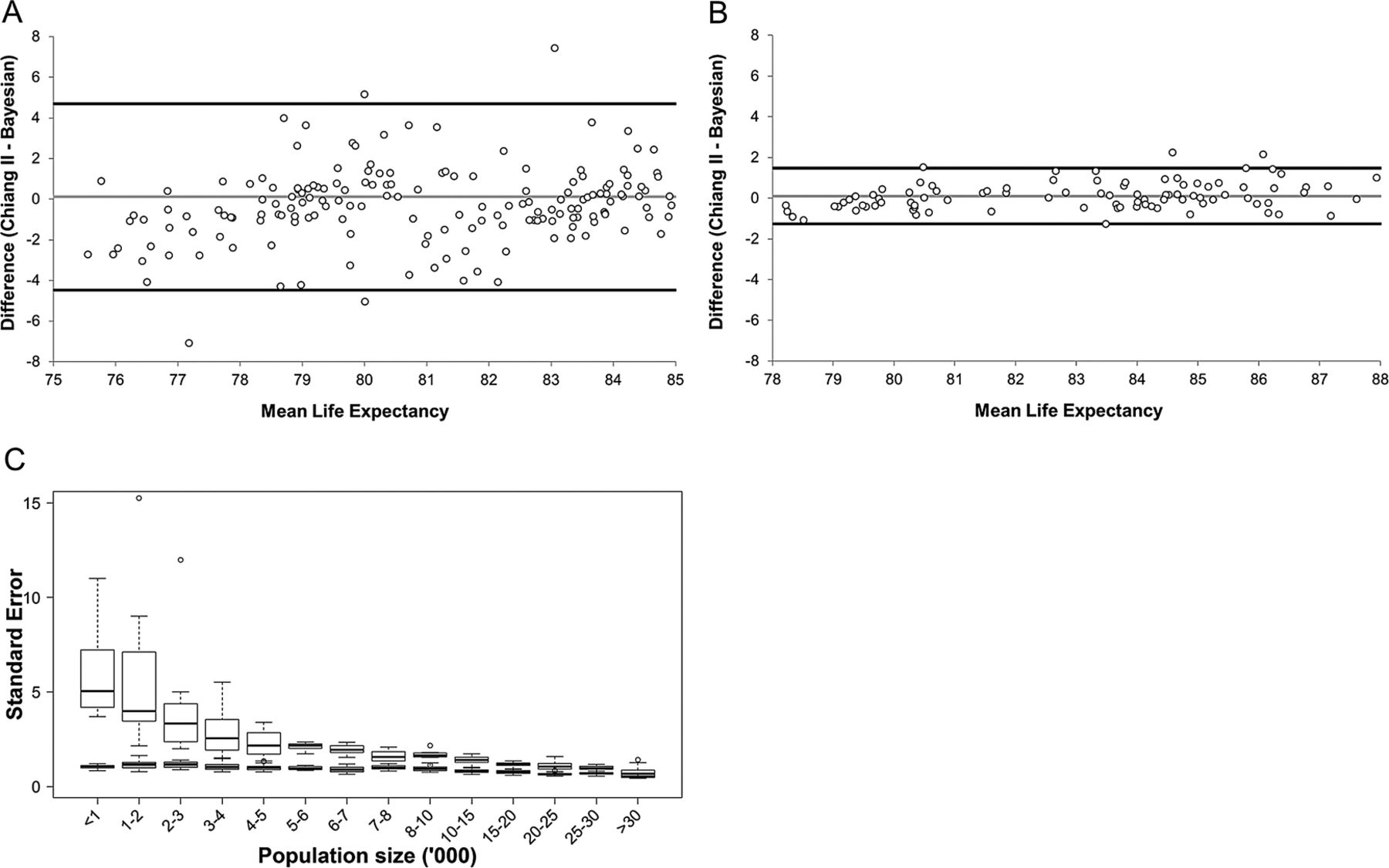
NSW LGAs display a great diversity in population sizes (table 1) and deciding on a life expectancy estimation methodology that was suitable to small as well as large populations was a primary objective. Performance of the Chiang II and Silcocks methods of life expectancy estimation in LGAs was compared in relation to agreement of estimates, SEs of life expectance estimates and rate of calculation failures with varying population sizes. The agreement analysis showed that the two methods produced almost identical life expectancy estimates at birth (figure 1A) and also at age 65 (figure 1B). However, the Silcocks method consistently produced marginally higher estimates at birth as well as age 65 (mean increases of 0.023 and 0.027 years, respectively). Larger differences in SEs were observed between the two methods (figure 1C). The Chiang II method consistently generated lower SEs and this effect was more pronounced in smaller populations. Conceivably, the decreased variance in Chiang II was due to the lack of variance contributed by the final age interval. Application of the Silcocks method of calculating variance in the final age interval to the Chiang II method (termed adjusted Chiang II) generated SEs that were almost identical to Silcocks. Based on the similar performance of the two methods, the widely applied Chiang II methodology adapted to include the Silcocks method of calculating variance for the final age interval (also proposed by Eayres and Williams5) was used for the remainder of the study.
Female and male NSW LGA population size frequencies

Comparison of Chiang II and Silcocks life expectancy estimates and standard errors. (A and B) Agreement analysis of Chiang II and Silcocks life expectancy estimates at birth (A) and at age 65 (B). (C) Chart of Chiang II, Silcocks and adjusted Chiang II standard errors over increasing population size revealing decreased variance in Chiang II. For (A and B) differences are represented by empty circles. Thick black lines represent upper and lower limits of agreement. The thin grey line represents the mean difference.
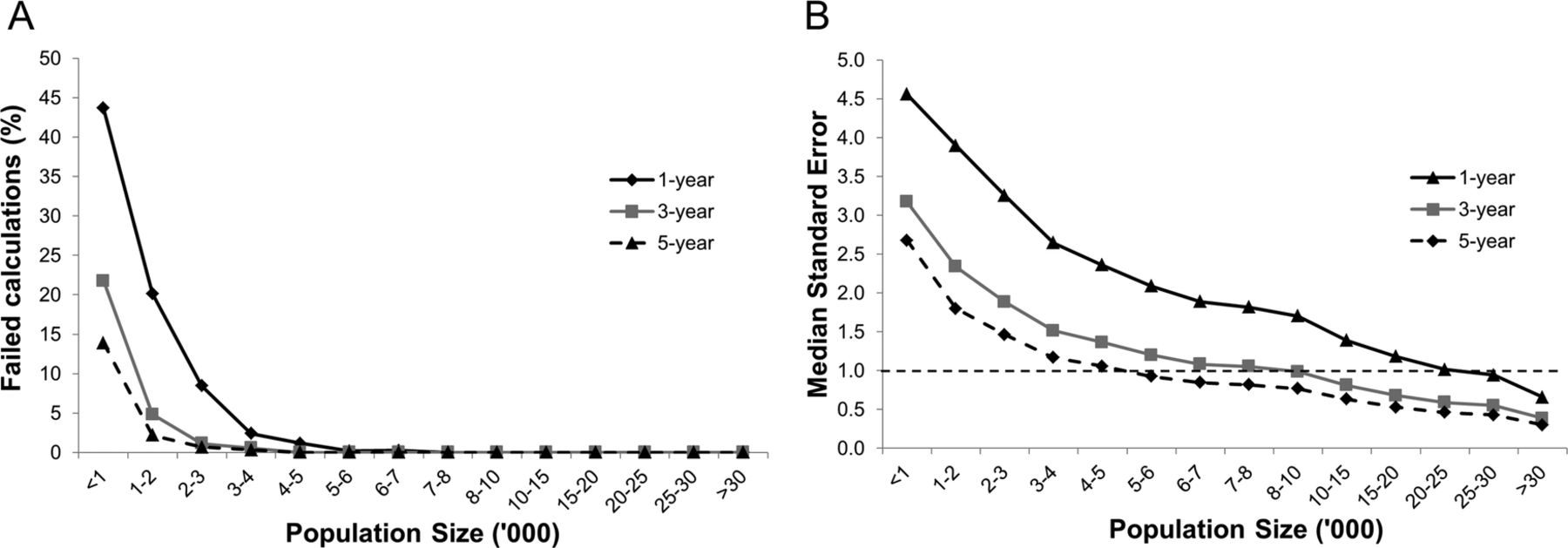
Chiang II and Silcocks methods fail in instances where there are zero deaths in the final age interval. Although the likelihood of recording zero deaths in the oldest age group, where the mortality rate is generally at its peak, is low in large populations, this likelihood will tend to rise with decreasing population size. We investigated the rates of life expectancy calculation failures with changing population size using the adjusted Chiang II method (figure 2A). When applying single year level data (no data aggregation), over 43% and approximately 20% of calculations failed in LGAs with populations less than 1000 and 1000–2000, respectively. The observed failure rate reached zero per cent in the 7000–8000 category. The effect of aggregating data over 3 or 5 years greatly improved the stability of calculations with zero failures observed in populations sized 4000–5000 or greater for 3 and 5 years data aggregation.

Percentage of failed calculations and median standard errors of life expectancy estimates as a function of sex-specific population size and years of data aggregation using adjusted Chiang II. (A) Percentage of failed calculations due to zero deaths in the final age interval. (B) Median standard errors of calculated life expectancy estimates. Dashed reference line represents a SE of 1 year. Results are displayed as a function of three different data aggregation categories based on the number of calendar years for which data was aggregated and used in calculations: 1, 3 and 5 years.
The SEs associated with life expectancy estimates was also investigated. SEs provide a fundamental measure of the reliability and usefulness of generated life expectancy estimates and is a key component in deciding the adjusted Chiang II minimum population threshold for reliable estimation. We suggest this population threshold occurs when SEs reach approximately 1 year and is the limit the NSW Ministry of Health will adopt for the reporting of LGA life expectancy estimates. Steady declines in median SEs were observed with increasing population size among the 153 LGAs (figure 2B). Consistently, aggregating data over 3 or 5 years enhanced the precision of estimates. Table 2 summarises the population sizes required to generate life expectancy estimates with SEs of 1, 2 or 3 years by varying degrees of data aggregation for NSW LGA data.
Population size ranges required to attain median standard errors of 1, 2 or 3 years with varying degrees of data aggregation for New South Wales and local government areas data
Comparison of adjusted Chiang II method and Bayesian random effects model of life expectancy estimation
Studies have demonstrated that traditional life expectancy methods suffer from significant limitations in small populations and our own investigation of estimate reliability with varying population size provided further supporting evidence. To this end, we explored the Bayesian random effects model proposed by Jonker et al,7 as an alternative method to calculate life expectancy. The Bayesian random effects model was able to compute life expectancy estimates in all NSW LGAs irrespective of population size and this ‘freedom’ from calculation failures is a clear advantage over traditional approaches. We compared adjusted Chiang II estimates to those generated using the Bayesian model at two population categories (25 000 or below and above 25 000, figure 3A,B). The scatter plots showed relatively good agreement in populations over 25 000. However, agreement levels were considerably poorer in populations of 25 000 or less, reflecting the increased variance of adjusted Chiang II estimates in smaller populations. Mean differences of 0.11 (SD=2.32) and 0.11 (SD=0.70) for populations of 25 000 or less and greater than 25 000, respectively, did not suggest any systematic difference between the two methods at either population size.
Agreement between adjusted Chiang II and Bayesian derived life expectancy estimates for different sized populations and distributions of life expectancy estimate standard errors over increasing population size for adjusted Chiang II and Bayesian methods. (A) Agreement between adjusted Chiang II and Bayesian life expectancy methods in populations of 25 000 or less. (B) Agreement between Chiang II and Bayesian life expectancy methods in areas with populations above 25 000. For (A and B) differences are represented by empty circles. Thick black lines represent upper and lower limits of agreement. The thin grey line represents the mean difference. (C) Distributions of SEs for adjusted Chiang II and Bayesian derived estimates. White filled box plots indicate Chiang II estimate SEs and grey filled box plots indicate Bayesian estimate SEs. Empty circles represent outlier observations.
The next facet of comparing the methods was to assess the precision of life expectancy estimates across a range of population sizes (figure 3C). Bayesian model SEs were markedly lower compared with the adjusted Chiang II method in areas with populations below 10 000. Bayesian model SEs were also lower for all remaining population size categories investigated, however the size of the differences in SEs between the two methods lessened with increasing population size. At population size categories of 25 000–30 000 and 30 000 or greater, adjusted Chiang II median SEs were only marginally larger by 0.27 and 0.15 years, respectively, compared with Bayesian model median SEs.
Discussion
Accurate derivation of life expectancy across a diverse range of population sizes is necessary to support the planning and funding of healthcare services by government agencies across different administrative geographic boundaries. We compared the Chiang II and Silcocks methods of life expectancy estimation in 153 small government areas of NSW. The analysis demonstrated that the methods generated similar estimates across the different sized LGAs and supported the observations of Eayres and Williams, which also showed good agreement between the two methods.5 However, a notable difference was the reduced variance of Chiang II estimates. Adjustment of the Chiang II method by applying the Silcocks version of calculating variance for the final age interval accounted for the lowered variance. We believe that this composite method, termed adjusted Chiang II, generates accurate estimates with an improved measure of uncertainty by incorporating variance for all age intervals. This composite methodology was also proposed by Eayres and Williams which selected Chiang II in preference over Silcocks as the former method more accurately estimated Government Actuaries Department life expectancy.5 The performance of the adjusted Chiang II method across several population categories was tested and showed that calculation failures and large SEs became significant problems in small populations. Our results agreed with previously published reports which have also outlined the limitations of traditional methods.4–7
Performance analysis also served to identify the population threshold where the adjusted Chiang II methodology produced reliable estimates. For NSW LGA data, the population size required to completely avoid calculation failures was around 7000–8000. However, for policy and planning purposes, the preference of the NSW Ministry of Health is to report life expectancy estimates with a precision of 1 year or less. We understand that this is a subjective decision and other health administrations are at the liberty to choose their own limit of precision. Furthermore, the population sizes required to achieve SEs of 1, 2 and 3 years reported in this study were based entirely on NSW LGA data. It is likely that these limits might be different in other countries or even other Australian states where different age-specific mortality rates could lead to different SEs. Based on NSW LGA data, a population size of approximately 25 000 was required to achieve an SE of approximately 1 year using adjusted Chiang II. At this population size, estimates should be relatively free from overestimation bias,4 ,5 ,7 and we selected this population as the limit for calculating life expectancy using adjusted Chiang II. Aggregating data over 3 or 5 years beneficially reduced calculation failures and improved the precision of life expectancy estimates. However, a restraint of data aggregation over time is that calculated estimates will not reflect the most current and up to date conditions, rather they are more indicative of the mid-point of the period spanning the years over which data was aggregated. Data can also be aggregated across geographical areas but such aggregation would decrease area specificity, conflicting with the primary aim of small population estimation.
In light of traditional life expectancy method limitations, we applied the Bayesian random effects model for the calculation of life expectancy in NSW LGAs with the specific focus of deriving more precise estimates in populations of 25 000 and below. Through simulations, Jonker et al7 showed that the Bayesian method was superior to Chiang II in small populations in terms of bias, SEs and coverage of SEs and the large differences observed between adjusted Chiang II and Bayesian estimates in populations of 25 000 or less (based on agreement analysis of NSW LGA data) provided empirical evidence to support the high variability and bias of Chiang II estimates in small populations. For populations larger than 25 000, agreement between the two methods was much higher and reflected the fact that adjusted Chiang II estimates were more precise and should have been largely free from bias. It is important to note that Bayesian estimates remained more precise in the larger populations but the differences in precision between the two estimation methods were minor (eg, median SE was approximately 0.27 years larger for adjusted Chiang II in populations ranging between 25 000 and 30 000 compared with the Bayesian model) and the practical significance of these differences are small. The point at which adjusted Chiang II and the Bayesian approach display equal performance is yet to be defined, as simulations in Jonker et al,7 did not extend beyond 25 000, but based on extrapolation is likely to be between 25 000 and 75 000.
We feel that for populations of 25 000 or greater, either the Bayesian approach or adjusted Chiang II could be used to estimate life expectancy. The advantage of the Bayesian approach is that it is statistically superior (more precise) and this superiority could apply to populations of up to 75 000. The advantages of applying adjusted Chiang II in populations above 25 000 are that the method is widely used, well-accepted and is easier to explain to local health authorities. Furthermore, the use of adjusted Chiang II will guard against potential over-smoothing in areas where the assumption of spatial correlation is invalid. Balancing the gain in precision obtained using the Bayesian model and the simplicity and comparability of adjusted Chiang II we elected to apply adjusted Chiang II for the calculation of life expectancy in NSW LGAs with population sizes of greater than 25 000.
The main strength of this study is that the proposed hybrid method for calculating life expectancy for public reporting reflects common and accepted use among government agencies by employing the adjusted Chiang II for larger populations, while implementing the recently developed Bayesian approach to obtain more precise estimations for small populations. The approach can be readily implemented based on a population threshold of 25 000 (or similar). The methods maximise the utility of life expectancy estimates for population health monitoring and planning on a yearly basis while avoiding calculation failures, minimising SEs, limiting over-smoothing and reducing bias of estimates. The approach provides precise and recent estimates across geographic administrative areas of different sizes. The limitations of this study are that, while methodologically justifiable, it may be difficult for agencies to communicate the reasons why different methods are used for the same measure at the same administrative level (eg, local government areas) and that the use of the Bayesian method increases complexity.
In conclusion, we propose the use of a hybrid approach for the calculation of life expectancy in NSW LGAs. This approach consists of implementing a Bayesian random effects model in populations of 25 000 or less harnessing the improved precision obtained through intelligent Bayesian smoothing. For populations above 25 000, we elected to use the adjusted Chiang II method, which displayed a minor decrease in precision compared with the Bayesian approach but protects against bias if the assumption of spatial correlation is violated, has the advantage of being widely used, and is simpler to communicate to local health authorities.
Acknowledgments
The authors would like to thank Dr Marcel Jonker, Erasmus MC, University Medical Centre Rotterdam, for his expert advice on the Bayesian random effects model of life expectancy estimation and its implementation in WinBUGS 1.4.
Footnotes
-
Contributors ASS contributed to the design of the study, performed the data and statistical analysis, contributed to the interpretation of the results and was responsible for writing the manuscript and generating the tables and figures. SP contributed to the data analysis and interpretation of the study results and edited the manuscript. BY contributed to the design, analysis and interpretation of the study and participated in writing the manuscript. HM conceived and contributed to the design of the study, was centrally involved in the discussions of the results of the analysis and study outcomes, and assisted in the critical review of the manuscript.
-
Funding This work was supported by the NSW Ministry of Health.
-
Competing interests None.
-
Provenance and peer review Not commissioned; externally peer reviewed.
-
Data sharing statement No additional data are available.